8.1.1 Overview: Basic algorithms

8.1.1.1 k-nearest neighbor (k-NN)

k-NN is a non-parametric method used for classification and regression. Given an object, the algorithm’s output is computed from its k closest training examples in the feature space.

In k-NN classification, each object is classified into the class most common among its k nearest neighbors.
In k-NN regression, each object’s value is calculated as the average of the values of its k nearest neighbors.

Applications: anomaly detection, search, recommender system

8.1.1.2 k-means clustering

k-means clustering aims to partition observations into k clusters in which each observation belongs to the cluster with the nearest mean. k-means minimizes within-cluster variances (squared Euclidean distances), but not regular Euclidean distances.

The algorithm doesn’t guarantee convergence to the global optimum. The result may depend on the initial clusters. As the algorithm is usually fast, it is common to run it multiple times with different starting conditions.

The problem is computationally difficult (NP-hard); however, efficient heuristic algorithms converge quickly to a local optimum.

The algorithm has a loose relationship to the k-nearest neighbor classifier. After obtaining clusters using k-means clustering, we can classify new data into those clusters by applying the 1-nearest neighbor classifier to the cluster centers.

Applications: Vector quantization for signal processing (where k-means clustering was originally developed), cluster analysis, feature learning, topic modeling.

8.1.1.3 EM (expectation-maximization) algorithm

EM algorithm is an iterative method to find maximum likelihood (MLE) or maximum a posteriori (MAP) estimates of parameters. It’s useful when the model depends on unobserved latent variables and equations can’t be solved directly.

The iteration alternates between performing:

an expectation (E) step, which creates a function for the expectation of the log-likelihood evaluated using the current estimate for the parameters
a maximization (M) step, which computes parameters maximizing the expected log-likelihood found on the E step. These parameter-estimates are then used to determine the distribution of the latent variables in the next E step.

EM algorithm is guaranteed to return a local optimum of the sample likelihood function.

Example: Gaussian mixture models (GMM)

Applications: Data clustering, collaborative filtering.

8.1.1.4 Tree-based methods

Decision tree is a tree-based method that goes from observations about an object (represented in the branches) to conclusions about its target value (represented in the leaves). At its core, decision trees are nest if-else conditions.

In classification trees, the target value is discrete and each leaf represents a class. In regression trees, the target value is continuous and each leaf represents the mean of the target values of all objects that end up with that leaf.

Decision trees are easy to interpret and can be used to visualize decisions. However, they are overfit to the data they are trained on -- small changes to the training set can result in significantly different tree structures, which lead to significantly different outputs.

8.1.1.5 Bagging and boosting

Bagging and boosting are two popular ensembling methods commonly used with tree-based algorithms that can also be used for other algorithms.

8.1.1.5.1 Bagging

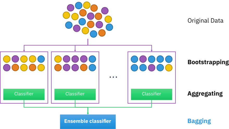
Bagging, shortened for bootstrap aggregating, is designed to improve the stability and accuracy of ML algorithms. It reduces variance and helps to avoid overfitting.

Given a dataset, instead of training one classifier on the entire dataset, you sample with replacement to create different datasets, called bootstraps, and train a classification or regression model on each of these bootstraps. Sampling with replacement ensures each bootstrap is independent of its peers.

If the problem is classification, the final prediction is decided by the majority vote of all models. For example, if 10 classifiers vote SPAM and 6 models vote NOT SPAM, the final prediction is SPAM.

If the problem is regression, the final prediction is the average of all models’ predictions.

Bagging generally improves unstable methods, such as neural networks, classification and regression trees, and subset selection in linear regression. However, it can mildly degrade the performance of stable methods such as k-nearest neighbors².

Illustration by Sirakorn

A random forest is an example of bagging. A random forest is a collection of decision trees constructed by both bagging and feature randomness, each tree can pick only from a random subset of features to use.

Due to its ensembling nature, random forests correct for decision trees’ overfitting to their training set.

Applications: Random forests are among the most widely used machine learning algorithms in the real world. They are used in banking for fraud detection, medicine for disease prediction, stock market analysis, etc.

For more information on random forests, see Understanding Random Forest by Tony Yiu.

8.1.1.5.2 Boosting

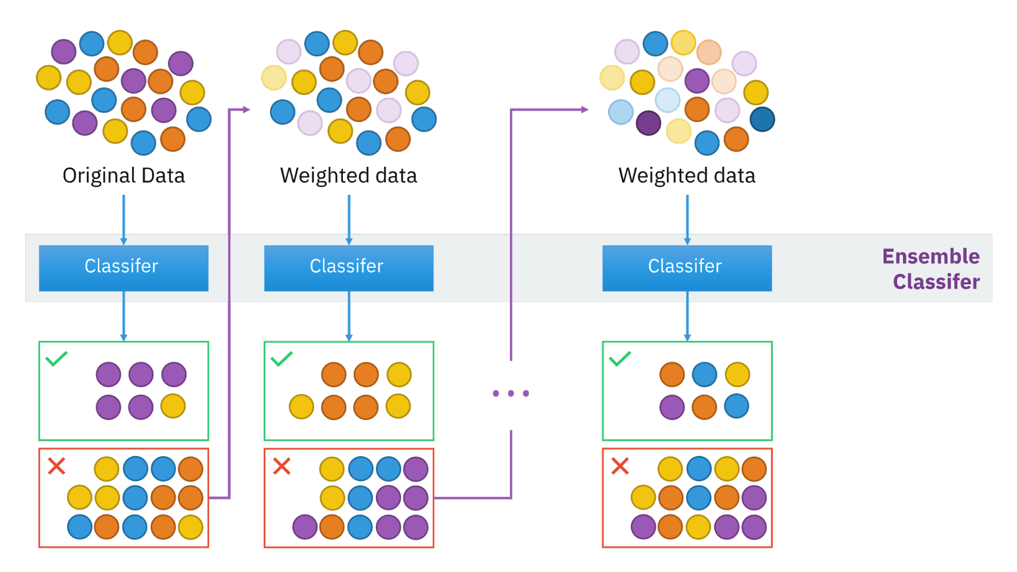
Boosting is a family of iterative ensemble algorithms that convert weak learners to strong ones. Each learner in this ensemble is trained on the same set of samples but the samples are weighted differently among iterations. Thus, future weak learners focus more on the examples that previous weak learners misclassified.

You start by training the first weak classifier on the original dataset.
Samples are reweighted based on how well the first classifier classifies them, e.g. misclassified samples are given higher weight.
Train the second classifier on this reweighted dataset. Your ensemble now consists of the first and the second classifiers.
Samples are weighted based on how well the ensemble classifies them.
Train the third classifier on this reweighted dataset. Add the third classifier to the ensemble.
Repeat for as many iterations as needed.
Form the final strong classifier as a weighted combination of the existing classifiers -- classifiers with smaller training errors have higher weights.

Illustration by Sirakorn

An example of a boosting algorithm is Gradient Boosting Machine which produces a prediction model typically from weak decision trees. It builds the model in a stage-wise fashion as other boosting methods do, and it generalizes them by allowing optimization of an arbitrary differentiable loss function.

XGBoost, a variant of GBM, used to be the algorithm of choice for many winning teams of machine learning competitions. It’s been used in a wide range of tasks from classification, ranking, to the discovery of the Higgs Boson³. However, many teams have been opting for LightGBM, a distributed gradient boosting framework that allows parallel learning which generally allows faster training on large datasets.

8.1.1.6 Kernel methods

In machine learning, kernel methods are a class of algorithms for pattern analysis, whose best-known member is the support vector machine (SVM). The general task of pattern analysis is to find and study general types of relations (for example clusters, rankings, principal components, correlations, classifications) in datasets. For many algorithms that solve these tasks, the data in raw representation have to be explicitly transformed into feature vector representations via a user-specified feature map: in contrast, kernel methods require only a user-specified kernel, i.e., a similarity function over pairs of data points in raw representation.

Kernel methods owe their name to the use of kernel functions, which enable them to operate in a high-dimensional, implicit feature space without ever computing the coordinates of the data in that space, but rather by simply computing the inner products between the images of all pairs of data in the feature space. This operation is often computationally cheaper than the explicit computation of the coordinates. This approach is called the "kernel trick".[1] Kernel functions have been introduced for sequence data, graphs, text, images, as well as vectors.

Algorithms capable of operating with kernels include the kernel perceptron, support vector machines (SVM), Gaussian processes, principal components analysis (PCA), canonical correlation analysis, ridge regression, spectral clustering, linear adaptive filters, and many others. Any linear model can be turned into a non-linear model by applying the kernel trick to the model: replacing its features (predictors) with a kernel function.

8.1.1 Overview: Basic algorithm