Introduction to streaming for data scientists
As machine learning moves towards real-time, streaming technology is becoming increasingly important for data scientists. Like many people coming from a machine learning background, I used to dread streaming. In our recent survey, almost half of the data scientists we asked said they would like to move from batch prediction to online prediction but can’t because streaming is hard, both technically and operationally. Phrases that the streaming community take for granted like “time-variant results”, “time travel”, “materialized view” certainly don’t help.
Over the last year, working with a co-founder who’s super deep into streaming, I’ve learned that streaming can be quite intuitive. This post is an attempt to rephrase what I’ve learned.
With luck, as a data scientist, you shouldn’t have to build or maintain a streaming system yourself. Your company should have infrastructure to help you with this. However, understanding where streaming is useful and why streaming is hard could help you evaluate the right tools and allocate sufficient resources for your needs.
Quick recap: historical data vs. streaming data
Once your data is stored in files, data lakes, or data warehouses, it becomes historical data.
Streaming data refers to data that is still flowing through a system, e.g. moving from one microservice to another.
Batch processing vs. stream processing Historical data is often processed in batch jobs — jobs that are kicked off periodically. For example, once a day, you might want to kick off a batch job to generate recommendations for all users. When data is processed in batch jobs, we refer to it as batch processing. Batch processing has been a research subject for many decades, and companies have come up with distributed systems like MapReduce and Spark to process batch data efficiently.
Stream processing refers to doing computation on streaming data. Stream processing is relatively new. We’ll discuss it in this post.
1. Where is streaming useful in machine learning?
There are three places in the ML production pipeline where streaming can matter a lot: online prediction, real-time observability, and continual learning.
Online prediction (vs. batch prediction)
Batch prediction means periodically generating predictions offline, before prediction requests arise. For example, every 4 hours, Netflix might generate movie recommendations for all of its users. The recommendations are stored and shown to users whenever they visit the website.
Online prediction means generating predictions on-demand, after prediction requests arise. For example, an ecommerce site might generate product recommendations for a user whenever this user visits the site. Because recommendations are generated online, latency is crucial.
Imagine you work for an ecommerce site and want to predict the optimal discount to give a user for a given product to encourage them to buy it. One of the features you might use is the average price of all the items this user has looked at in the last 30 minutes. This is an online feature – it needs to be computed on online data (as opposed to being pre-computed on historical data).
One “easy” way to do this is to spin up a service like AWS Lambda and Google Cloud Function to compute this feature whenever requests arrive. This is how many companies are doing it and it works in many simple cases. However, it doesn’t scale if you want to use complex online features.
This “easy” way is stateless, which means that each computation is independent from the previous one. Every time you compute this feature, you have to process all the data from the last 30 minutes, e.g:
- To compute this feature at 10:33am, you’ll have to process data from 10:03 to 10:33.
- To compute this feature again at 10:35, you’ll have to process data from 10:05 to 10:35.
The data from 10:05 to 10:33 is processed twice!
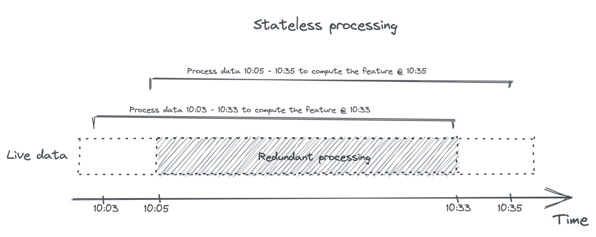
Stream processing can be stateless too, but stateless stream processing is kinda boring, so we’ll only talk about stateful stream processing here. Stateful stream processing can avoid redundancy, hence faster and cheaper. For example, when computing this feature again at 10:35, you’ll only need to process data from 10:33 to 10:35 and join the new result with the previous result.
Real-time monitoring (vs. batch monitoring)
There’s a world of difference between batch monitoring and real-time monitoring, and many monitoring solutions (especially batch solutions) conflate the two.
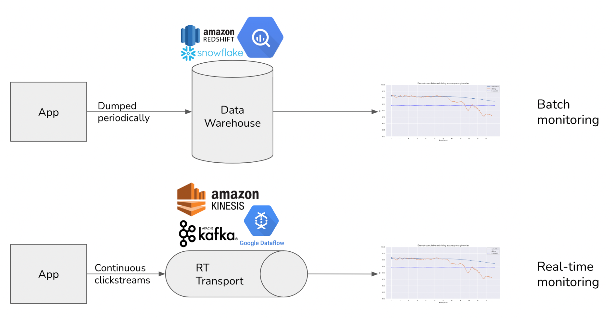
Batch monitoring means running a script to compute the metrics you care about periodically (like once a day), usually on data in warehouses like S3, BigQuery, Snowflake, etc. Batch monitoring is slow. You first have to wait for data to arrive at warehouses, then wait for the script to run. If your new model fails upon deployment, you won’t find out at least until the next batch of metrics is computed, assuming the metrics computed are sufficient to uncover the issue. And you can’t fix the failure before you find out about it.
Real-time monitoring means computing metrics on data as it arrives, allowing you to get insights into your systems in (near) real-time. Like online feature computation, real-time metric computation can often be done more efficiently with streaming.
If batch monitoring works for you, that’s great. In most use cases, however, batch monitoring often ends up being not enough. In software engineering, we know that the iteration speed is everything – cue Boyd’s Law of Iteration: speed of iteration beats quality of iteration. The DevOps community has been obsessed with speeding up iterations for higher quality software for over two decades. Two important metrics in DevOps are:
- MTTD: mean time to detection
- MTTR: mean time to response
If something is going to fail, you want it to fail fast, and you want to know about it fast, especially before your customers do. If your user has to call you in the middle of the night complaining about a failure or worse, tweet about it, you’re likely to lose more than one customer.
Yet, most people doing MLOps are still okay with day-long, even week-long feedback loops.
Many teams, without any monitoring system in place for ML, want to start with batch monitoring. Batch monitoring is still better than no monitoring, and arguably easier to set up than real-time monitoring.
However, batch monitoring isn’t a prerequisite for real-time monitoring – setting up batch monitoring today is unlikely to make it easier to set up real-time monitoring later. Working on batch monitoring first means another legacy system to tear down later when you need to get real-time.
Continual learning (vs. manual retraining)
Continual learning refers to the ability to update your models whenever needed and to deploy this update quickly. Fast model updates enable our models to adapt to changing environments and business requirements, especially to data distribution shifts.
I’ve talked to ML engineers / data scientists at over 100 companies. Almost everyone told me that continual learning is too “far out”. Most companies are still struggling with dependency management and monitoring to think about continual learning.
At the same time, nobody has ever told me that they don’t want continual learning. Continual learning is too “far out” because we don’t yet have the right tool for it. When the right tool emerges that makes continual learning “just work”, I believe the transition will be swift.
We don’t need streaming to continually update our models. Assuming that you already have a way of accessing fresh data, the hard part of continual learning isn’t in updating the models, but in ensuring that the updated models work. We need to find a way to evaluate each model iteration fast, which brings us back to real-time monitoring and streaming.
2. From table to log
I hope that I’ve convinced you why and where we need streaming in ML. If you’re not convinced, I’d love to hear from you. Now, let’s walk through some of the core concepts behind streaming that I find really cool.
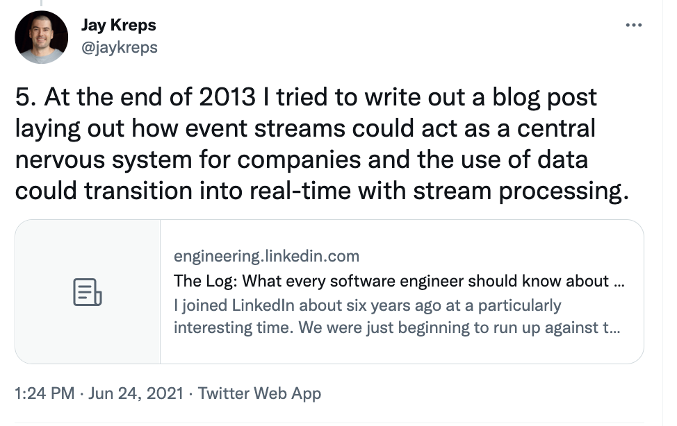
The first article that helped me make sense of streaming is the classic post The log by Jay Kreps, a creator of Kafka. Side note: Kreps mentioned in a tweet that he wrote the post to see if there was enough interest in streaming for his team to start a company around it. The post must have been popular because his team spun out of LinkedIn to become Confluent.
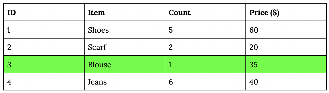
The core idea of the post (for me) is the duality of table and log. You’re probably already familiar with data tables, like a MySQL table or a pandas DataFrame. For simplicity, consider the following inventory table.
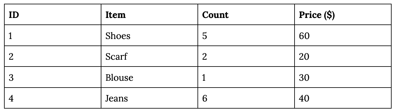
Let’s say, on June 19, you want to make a change to this table – e.g. changing the price of item #3 (Blouse) from $30 to $35. There are many ways to do this, but the 2 common approaches are:
- Go to where the table is stored and make the change directly (e.g. overwriting a file). This means that we’ll have no way of reverting the change, but many companies do it anyway.
- Send an update with the new price
{"timestamp": "2022-06-19 09:23:23", "id": 3, "Price ($)": 35}, and this update will be applied to the table. Overtime, we’ll have a series of ordered updates, which is called a log. Each update is an example of an event. Logs are append-only. You can only append the new events to your existing log. You can’t overwrite previous events.
…
{"timestamp": "2022-06-08 11:05:04", "id": 3, "Item": "Blouse", "Price ($)": 30}
{"timestamp": "2022-06-17 03:12:16", "id": 4, "Item": "Jeans", "Price ($)": 40}
{"timestamp": "2022-06-19 09:23:23", "id": 3, "Item": "Blouse", "Price ($)": 35}
I’m using wall clock timestamps for readability. In practice, wall clocks are unreliable. Distributed systems often leverage logical clock instead.
A table captures the state of data at a point in time. Given a table alone, we don’t know what the state of data was a day ago or a week ago. Given a log of all the changes to this table, we can recreate this table at any point in time.
You’re already familiar with logs if you work with git. A git log keeps track of all the changes to your code. Given this log, you can recreate your code at any point in time.
Stateless vs. stateful log
It’s possible to send an event with the price difference only {"id": 3, "Action": "increase", "Price ($)": 5}. For this type of event we’ll need to look at the previous price to determine the updated price.
This is called a stateful event (we need to know the previous state to construct the current state). The type of event mentioned in #2 is a stateless log. Stateful events are required to be processed in order – adding $5 to the blouse price then doubling it is very different from doubling it then adding $5.
There’s a whole industry focusing on solving stateful events called Change Data Capture (CDC). See Debezium, Fivetran, Striim.
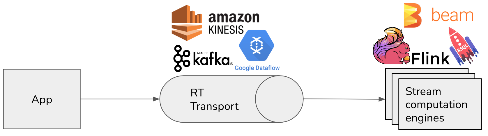
Real-time transport and computation engine
There are two components of a streaming system: the real-time transport and the computation engine.
- The real-time transport, which are basically distributed logs. Data in real-time transports are called streaming data, or “data in motion” as coined by Confluent. Examples: Kafka, AWS Kinesis, GCP Dataflow.
- The computation engine performs computation (e.g. joining, aggregation, filtering, etc.) on the data being transported. Examples: Flink, KSQL, Beam, Materialize, Decodable, Spark Streaming.
Transports usually have capacity for simple computation. For example, Kafka is a transport that also has an API called Kafka Streams that provides basic stream processing capacity. However, if you want to perform complex computation, you might want an optimized stream computation engine (similar to how bars usually have some food options but if you want real food you’ll want to go to a restaurant).
We’ve discussed logs at length. From the next section onward, we’ll focus on stream computation.
3. A simple example of stream processing
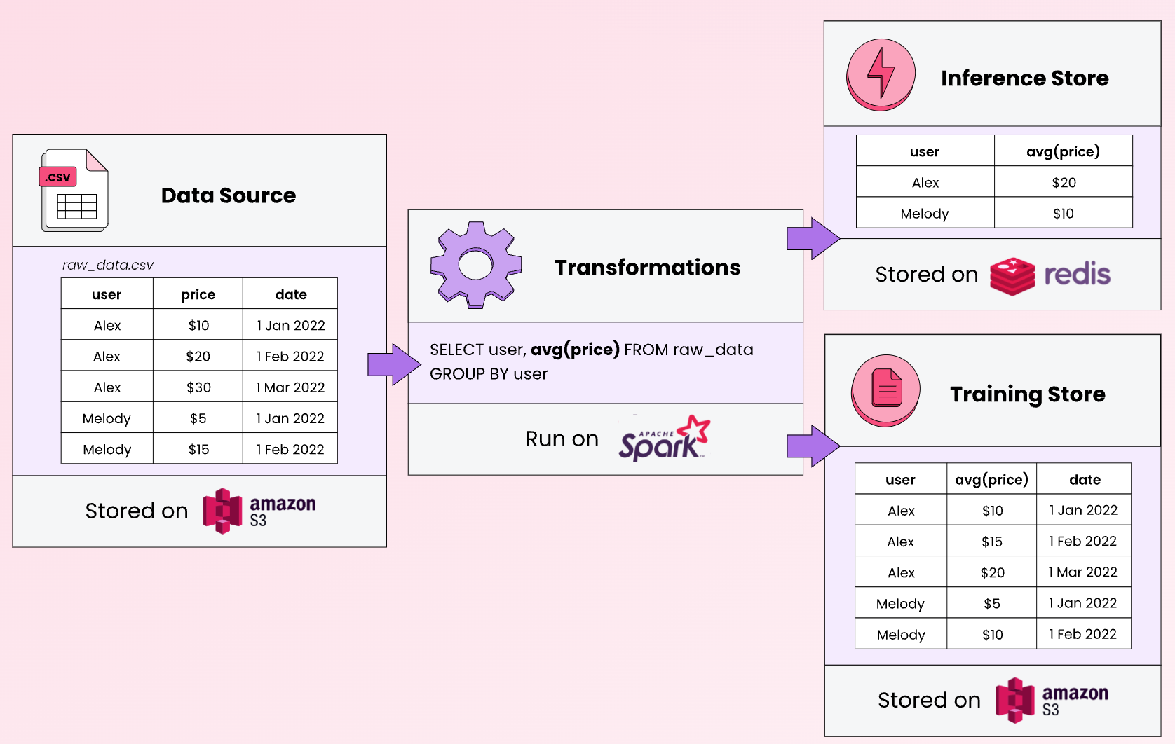
Imagine that we want to use the average price of all items a user has looked at as a feature. If we put all these items into a table, the feature definition might look something like this. This is batch processing.
# Pseudocode
def average_price(table):
    return sum(table.price) / len(table)
If, instead, we have a log of all item updates, how should we compute the average price?
Internal state and checkpoints
One way to do it is to process events in the log (replay the log) from the beginning of time to recreate the inventory table of all items. However, we actually don’t need to keep track of the whole table to get the average price – we just need the total price of all items and the item count. The average price can be computed from these two values.
The total price and the count constitute the internal state of the stream processing job. We say this computation is stateful because we keep track of the internal state between computation.
# Pseudocode
def average_price(log):
    initialize total_price, item_count
    for each event in the log:
        update total_price, item_count
    avg_price = total_price / item_count
return avg_price
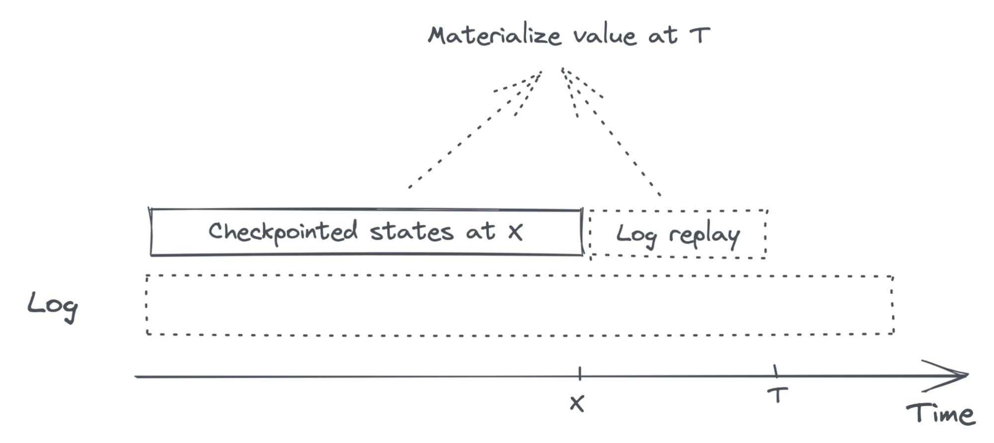
If the log is large (in 2021, Netflix was processing 20 trillion events a day!), replaying the log from the beginning can be prohibitively slow. To mitigate this, we can occasionally save the internal state of the job, e.g. once every hour. The saved internal state is called a checkpoint (or savepoint), and this job can resume from any checkpoint. The function above will be updated as follows:
# Pseudocode
def average_price(log):
    find the latest checkpoint X
    load total_price, item_count from X
    for each event in the log after X:
update total_price, item_count
avg_price = total_price / item_count
return avg_price
Materialized view
The computed average price value, if saved, will become a materialized view of the feature average price. Each time we query from the materialized view, we don’t recompute the value, but read the saved value.
You might wonder: “Why must we come up with a new term like materialized view instead of saying saved copy or cache?”
Because “saved copy” or “cache” implies that the computed value will never change. Materialized views can change due to late arrivals. If an event that happened at 10.15am got delayed and arrived at 11.10am, all the materialized views that might be affected by this update should be recomputed to account for this delayed event. I say “should” because not all implementations do this.
Reading from a materialized view is great for latency, since we don’t need to recompute the feature. However, the materialized view will eventually become outdated. Materialized views will need to be refreshed (recomputed) either periodically (every few minutes) or based on a change stream.
When refreshing a materialized view, you can recompute it from scratch (e.g. using all the items to compute their average price). Or you can update it using only the new information (e.g. using the latest materialized average price + the prices of updated items). The latter is called incremental materialized. For those interested, Materialize has a great article with examples on materialized and incremental materialized.
4. Time travel and backfilling
We’ve talked about how to compute a feature on the latest data. Next, we’ll discuss how to compute a feature in the past.
Imagine that the latest price for the item blouse in our inventory is $35. We want to compute the avg_price feature as it would’ve happened on June 10. There are two ways this feature might have differed in the past:
- The data was different. For example, the blouse’s price was $30 instead of $35.
- The feature logic was different. For example:
- Today, the
avg_pricefeature computes the average raw price of all items. - On June 10, the
avg_pricefeature computes the average listed price, and the listed price is the raw price plus discount.
- Today, the
If we accidentally use the data or the feature logic from today instead of the data & logic from June 10, it means there is a leakage from the future. Point-in-time correctness refers to a system’s ability to accurately perform a computation as it would’ve happened at any time in the past. Point-in-time correctness means no data leakage.
Retroactively processing historical data using a different logic is also called backfilling. Backfilling is a very common operation in data workflows, e.g. see backfilling in Airflow and Amplitude. Backfilling can be done both in batch and streaming.
- With batch backfilling, you can apply the new logic (e.g. new feature definition) to a table in the past.
- With stream backfilling, you can apply the new logic to the log in a given period of time in the past, e.g. apply it to the log on June 10, 2022.
Time travel is hard, because we need to keep track of the states of your data over time. It can get very complicated if your data is joined from multiple places. For example, the average listed price depends on raw prices and discounts, both of them can independently change over time.
Time travel in ML workflows
There are many scenarios in an ML workflow where time travel is necessary, but here are the two major ones:
- to ensure the train-predict consistency for online features (also known as online-offline skew or training-serving skew)
- to compare two models on historical data
Train-predict consistency for online features
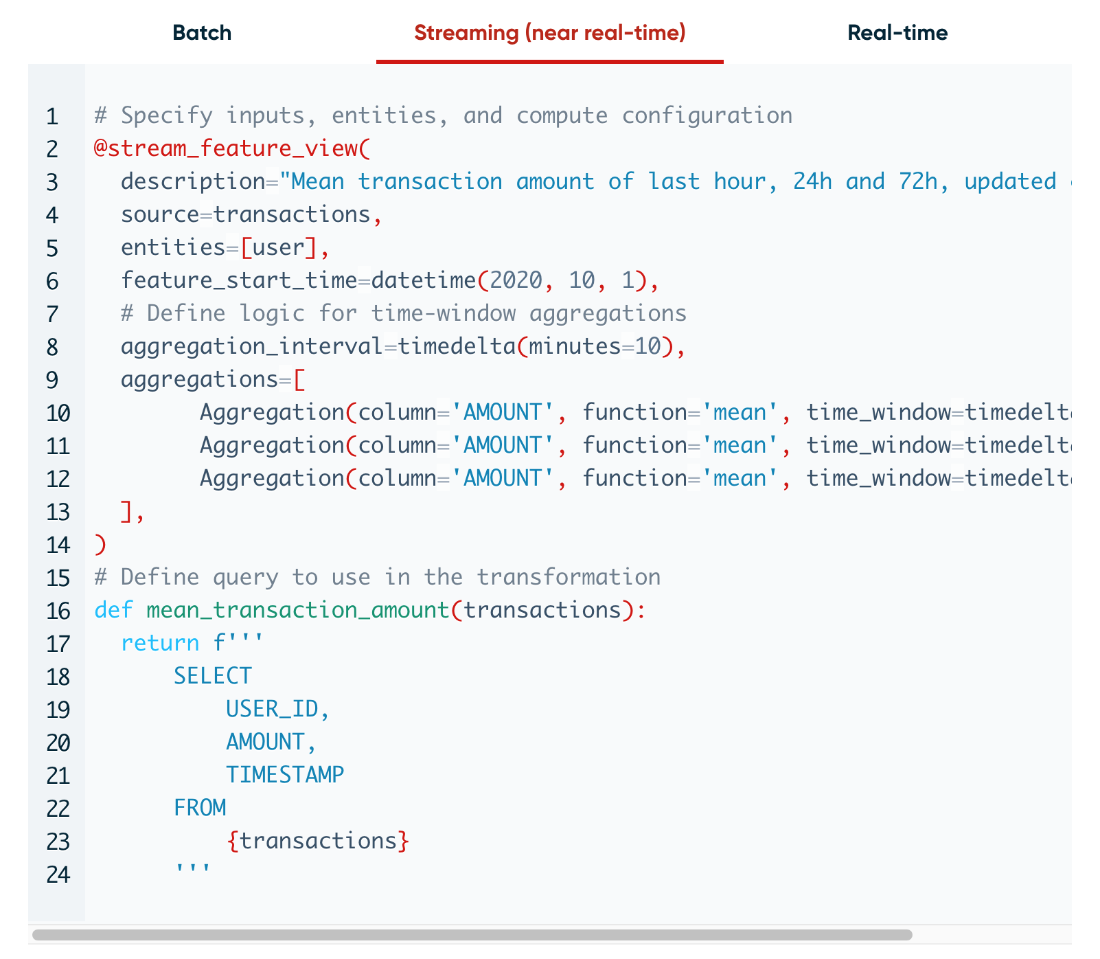
Online prediction can cause train-predict inconsistency. Imagine our model does online prediction using online features, one of them is the average price of all the items this user has looked at in the last 30 minutes. Whenever a prediction request arrives, we compute this feature using the prices for these items at that moment, possibly using stream processing.
During training, we want to use this same feature, but computed on historical data, such as data from the last week. Over the last week, however, the prices for many items have changed, some have changed multiple times. We need time travel to ensure that the historical average prices can be computed correctly at each given point in time.
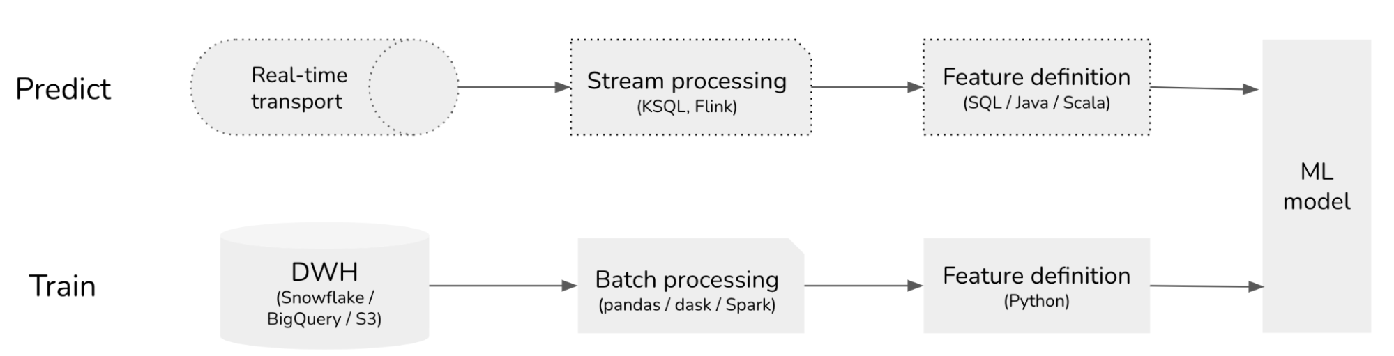
Production-first ML
Traditionally, ML workflows are development-first. Data scientists experiment with new features for the training pipeline. Feature definitions, aka feature logic, are often written for batch processing, blissfully unaware of the time-dependent nature of data. Training data often doesn’t even have timestamps.
This approach might help data scientists understand how a model or feature does during training, but not how this model / feature will perform in production, both performance-wise (e.g. accuracy, F1) and operation-wise (e.g. latency).
At deployment, ML or ops engineers need to translate these batch features into streaming features for the prediction pipeline and optimize them for latency. Errors during this translation process – e.g. changes or assumptions in one pipeline not updated or insufficiently tested in another – create train - predict inconsistency.
This inconsistency gets worse when the training and prediction pipelines use different languages, e.g. the training pipeline uses Python and the prediction pipeline uses SQL or Java.
To avoid this inconsistency, we should get rid of the translation process altogether. What if we let data scientists experiment with features for the prediction pipeline directly? You can write new features as they will be used in production. To test out these new features, you apply them to historical data to generate training data to train models. Applying new feature logic to historical data is exactly what backfilling is. With this setup, ML workflows become production-first!
Thanks to its ability to support both streaming and batch processing, SQL has emerged to be a popular language for production-first ML workflows. In the relational database era, SQL computation engines were entirely in the batch paradigm. In recent years, there has been a lot of investment in streaming SQL engines, such as KSQL and Apache Flink. (See Streaming SQL to Unify Batch & Stream Processing w/ Apache Flink @Uber)
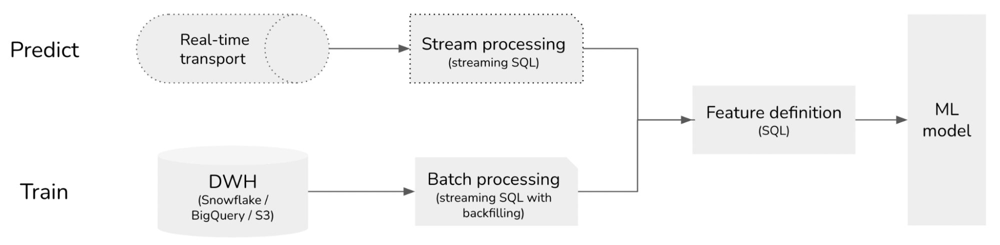
Development-first ML workflows: features are written for training and adapted for online prediction.
Production-first ML workflows: features are written for online prediction and backfilled for training.
Backtest for model comparison
Backfilling to generate features for training is how feature stores like FeatureForm and Tecton ensure train-predict consistency. However, most feature stores only support limited streaming computation engines, which can pose performance (latency + cost) challenges when you want to work with complex online features.
Imagine your team is using model A to serve live prediction requests, and you just came up with a new model B. Before A/B testing model B on live traffic, you want to evaluate model B on the most recent data, e.g. on the prediction requests from the last day.
To do so, you replay the requests from the last day, and use model B to generate predictions for those requests to see what the performance would have been if we had used B instead of A.
If model B uses exactly the same feature logic as model A, model B can reuse the features previously computed for model A. However, if model B uses a different feature set, you’ll have to backfill, apply model B’s feature logic to data from the last day, to generate features for model B.
This is also called a backtest.
Time travel challenges for data scientists
Some data science teams have told me that they need to do time travel for their data but their data doesn’t have timestamps. What should they do?
It’s impossible to time travel without timestamps. This is not a problem that data scientists can solve without having control over how data is ingested and stored.
So why don’t data scientists have access to data with timestamps?
One reason is that data platforms might have been designed using practices from an era where ML production wasn’t well understood. Therefore, they were not designed with ML production in mind, and timestamps weren’t considered an important artifact to keep track of.
Another reason is the lack of communication between those who ingest the data (e.g. the data platform team) and those who consume the data (e.g. the data science team). Many companies already have application logs, however, the timestamps are not retained during data ingestion or processing, or they are retained somewhere that data scientists don’t access to.
This is an operational issue that companies who want modern ML workflows will need to invest into. Without a well-designed data pipeline, data scientists won’t be able to build production-ready data applications.
the reason data quality is bad is because most data teams have zero power over the creation of data. it's like a soviet supply chain, where the end consumer has to accept whatever the factory churns out.
— Slater Stich (@slaterstich) June 1, 2022
5. Why is streaming hard?
I hope that by now, I’ve convinced you why streaming is important for ML workloads. Another question is: if streaming is so important, why is it not more common in ML workflows?
Because it’s hard.
If you’ve worked with streaming before, you probably don’t need any convincing. Tyler Aikidau gave a fantastic talk on the open challenges in stream processing. Here, I’ll go over the key challenges from my perspective as a data scientist. This is far from an exhaustive list. A streaming system needs to be able to handle all of these challenges and more.
Distributed computation
Streaming is simple when you have a small amount of updates and they are generated and consumed by one single machine, like the inventory example in From table to log. However, a real-world application can have hundreds, if not thousands, of microservices, spread out over different machines. Many of these machines might try to read and write from the same log. Streaming systems are highly distributed. Engineers working directly with streaming need to have a deep understanding of distributed systems, which not many data scientists would’ve exposure to in their day-to-day jobs. We need good abstraction to enable data scientists to leverage streaming without having to deal with the underlying distributed systems.
Time-variant results
Time adds another dimension of complexity. If you apply the same query to the same table twice, you’ll get the same result. However, if you apply the same query to the same stream twice, you’ll likely get very different results.
In batch, if a query fails, you can just rerun it. But in streaming, due to time-variant results, if a query fails, what should we do? Different stream processing engines have different ways to address this problem. For example, Flink uses the Chandy–Lamport algorithm, developed by K. Mani Chandy and the Turing Award winner Leslie Lamport.
Cascading failure
In a batch setting, jobs are typically scheduled at large intervals, hence fluctuation in workloads isn’t a big deal. If you schedule a job to run every 24 hours and one run takes 6 hours instead of 4 hours, these extra 2 hours won’t affect the next run.
However, fluctuation in a streaming setting can make it very hard to maintain consistently low latency. Assuming that your streaming system is capable of handling 100 events / second. If the traffic is less than 100 events / second, your system is fine. If the traffic suddenly surges to 200 events one second, ~100 events will be delayed. If not addressed quickly, these delayed 100 seconds will overload your system the next second, and so on, causing your system to significantly slow down.
Availability vs. consistency
Imagine that there are two machines trying to send updates about the same item:
- Machine A, at “03:12:10”, updates that user views product 123
- Machine B, at “03:12:16”, updates that user views product 234
Due to some network delays, machine A’s update is delayed in transit, and arrives later than machine B’s update. How long should we wait for machine A before computing the average prices of all items the user has looked at in the last 30 minutes?
If we don’t wait long enough, we’ll miss machine A’s update, and the feature will be incorrect. However, if we wait too long, the latency will be low. An optimal time window is probably somewhere in the middle. Therefore, the results of stream computation tend to be approximate.
This leads us to an interesting trade-off: availability vs. consistency. For our system to be highly available, we’ll want to duplicate the same workload over multiple machines. However, the more machines there are, the more stragglers there will be, and the more inconsistent the results of your stream computation will become. All large-scale distributed systems, not just streaming systems, have to make this tradeoff.
Operational challenges
While streaming technology can be technically hard, the real challenge for companies to adapt streaming is in operations. Operating on (near) real-time data streams means that we can make things happen in (near) real-time. Unfortunately, this means that catastrophes can also happen in (near) real-time.
Maintaining a streaming system means that your engineers will have to be on-call 24x7 to respond to incidents quickly. If you can’t figure out the problems and resolve them fast enough, data streams will be interrupted and you might lose data. Because the stake is higher in streaming systems, maintenance of streaming systems requires a high level of automation and mature DevOps practices.
We’ve talked to many small teams who want to maintain their own Kafka or Flink clusters and it’s not pretty. Streaming is an area where I can see a lot of values in managed services (e.g. Confluent instead of Kafka).
Conclusion
Wow, this was a hard post for me to write. I hope you’re still with me.
I’m very excited about the application of streaming for ML applications. My dream is that data scientists should have access to an ML platform that enables them to leverage streaming without having to worry about its underlying complexities. This platform needs to provide a high-enough level of abstraction for things to just work, while being flexible enough for data scientists to customize their workflows.
I know that leveraging streaming for ML is hard right now and I believe in the value of making it easier, so I’m working on it. Hit me up if you want to chat!
This is a relatively new field, and I’m still learning too. I’d appreciate any feedback and discussion points you have!
Acknowledgment
Thanks Zhenzhong Xu for having patiently answered all my dumb questions on streaming, Luke Metz, Chloe He, Han-chung Lee, Dan Turkel, and Robert Metzger.