Generation configurations: temperature, top-k, top-p, and test time compute
ML models are probabilistic. Imagine that you want to know what’s the best cuisine in the world. If you ask someone this question twice, a minute apart, their answers both times should be the same. If you ask a model the same question twice, its answer can change. If the model thinks that Vietnamese cuisine has a 70% chance of being the best cuisine and Italian cuisine has a 30% chance, it’ll answer “Vietnamese” 70% of the time, and “Italian” 30%.
This probabilistic nature makes AI great for creative tasks. What is creativity but the ability to explore beyond the common possibilities, to think outside the box?
However, this probabilistic nature also causes inconsistency and hallucinations. It’s fatal for tasks that depend on factuality. Recently, I went over 3 months’ worth of customer support requests of an AI startup I advise and found that ⅕ of the questions are because users don’t understand or don’t know how to work with this probabilistic nature.
To understand why AI’s responses are probabilistic, we need to understand how models generate responses, a process known as sampling (or decoding). This post consists of 3 parts.
- Sampling: sampling strategies and sampling variables including temperature, top-k, and top-p.
- Test time compute: increasing the compute allocated to inference, e.g. sampling multiple outputs, to help improve a model’s performance.
- Structured outputs: how to get models to generate outputs in a certain format.
Sampling
Given an input, a neural network produces an output by first computing the probabilities of all possible values. For a classifier, possible values are the available classes. For example, if a model is trained to classify whether an email is spam, there are only two possible values: spam and not spam. The model computes the probability of each of these two values, say being spam is 90% and not spam is 10%.
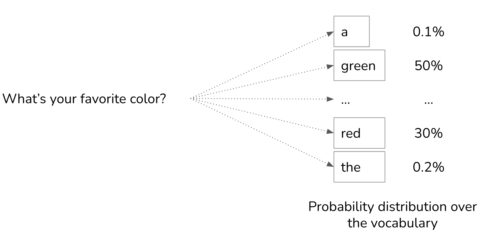
To generate the next token, a language model first computes the probability distribution over all tokens in the vocabulary.
For the spam email classification task, it’s okay to output the value with the highest probability. If the email has a 90% chance of being spam, you classify the email as spam. However, for a language model, always picking the most likely token, greedy sampling, creates boring outputs. Imagine a model that, for whichever question you ask, always responds with the most common words.
Instead of always picking the next most likely token, we can sample the next token according to the probability distribution over all possible values. Given the context of My favorite color is ..., if red has a 30% chance of being the next token and green has a 50% chance, red will be picked 30% of the time, and “green” 50% of the time.
Temperature
One problem with sampling the next token according to the probability distribution is that the model can be less creative. In the previous example, common words for colors like red, green, purple, etc. have the highest probabilities. The language model’s answer ends up sounding like that of a five-year-old: My favorite color is green. Because the has a low probability, the model has a low chance of generating a creative sentence such as My favorite color is the color of a still lake on a spring morning.
Temperature is a technique used to redistribute the probabilities of the possible values. Intuitively, it reduces the probabilities of common tokens, and as a result, increases the probabilities of rarer tokens. This enables models to create more creative responses.
To understand how temperature works, let’s take a step back to see how a model computes the probabilities. Given an input, a neural network processes this input and outputs a logit vector. Each logit corresponds to one possible. In the case of a language model, each logit corresponds to one token in the model’s vocabulary. The logit vector size is the size of the vocabulary.
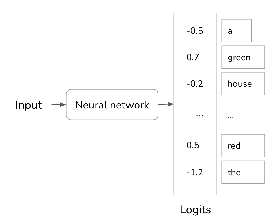
While larger logits correspond to higher probabilities, the logits don’t represent the probabilities. Logits don’t sum up to one. Logits can even be negative, while probabilities have to be non-negative. To convert logits to probabilities, a softmax layer is often used. Let’s say the model has a vocabulary of N and the logit vector is \([x_1, x_2, ..., x_N]\). The probability for the \(i^{th}\) token, \(p_i\), is computed as follows:
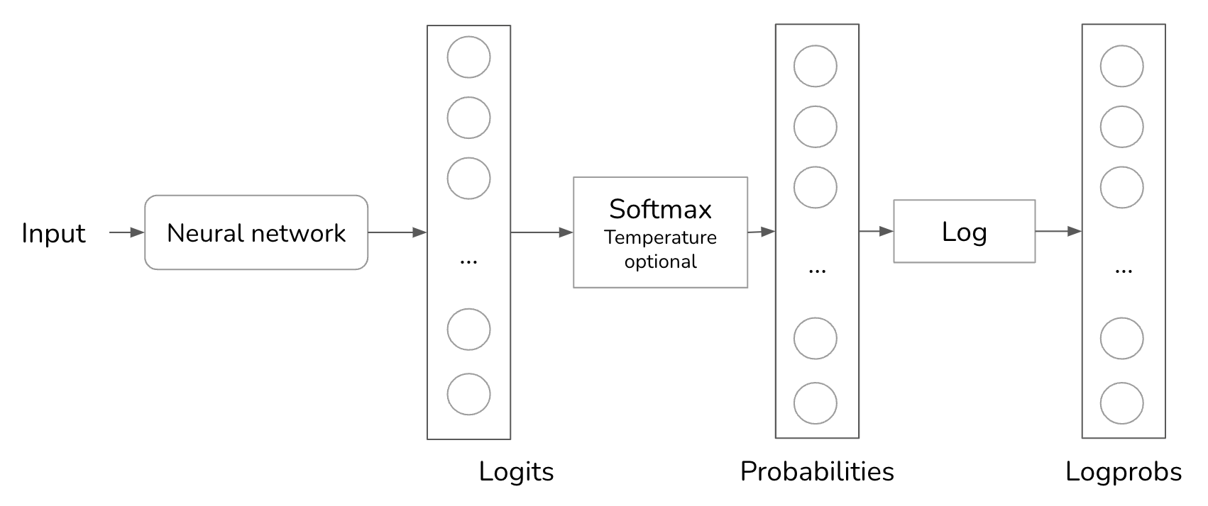
\[p_i = \text{softmax}(x_i) = \frac{e^{x_i}}{\sum_j e^{x_j}}\]Temperature is a constant used to adjust the logits before the softmax transformation. Logits are divided by temperature. For a given temperature of \(T\), the adjusted logit for the \(i^{th}\) token is \(\frac{x_i}{T}\). Softmax is then applied on this adjusted logit instead of on \(x_i\).
Let’s walk through a simple example to understand the effect of temperature on probabilities. Imagine that we have a model that has only two possible outputs: A and B. The logits computed from the last layer are [1, 3]. The logit for A is 1 and B is 3.
- Without using temperature, equivalent to temperature = 1, the softmax probabilities are
[0.12, 0.88]. The model picks B 88% of the time. - With temperature = 0.5, the probabilities are
[0.02, 0.98]. The model picks B 98% of the time. - With temperature = 2, the probabilities are
[0.27, 0.73]. The model picks B 73% of the time.
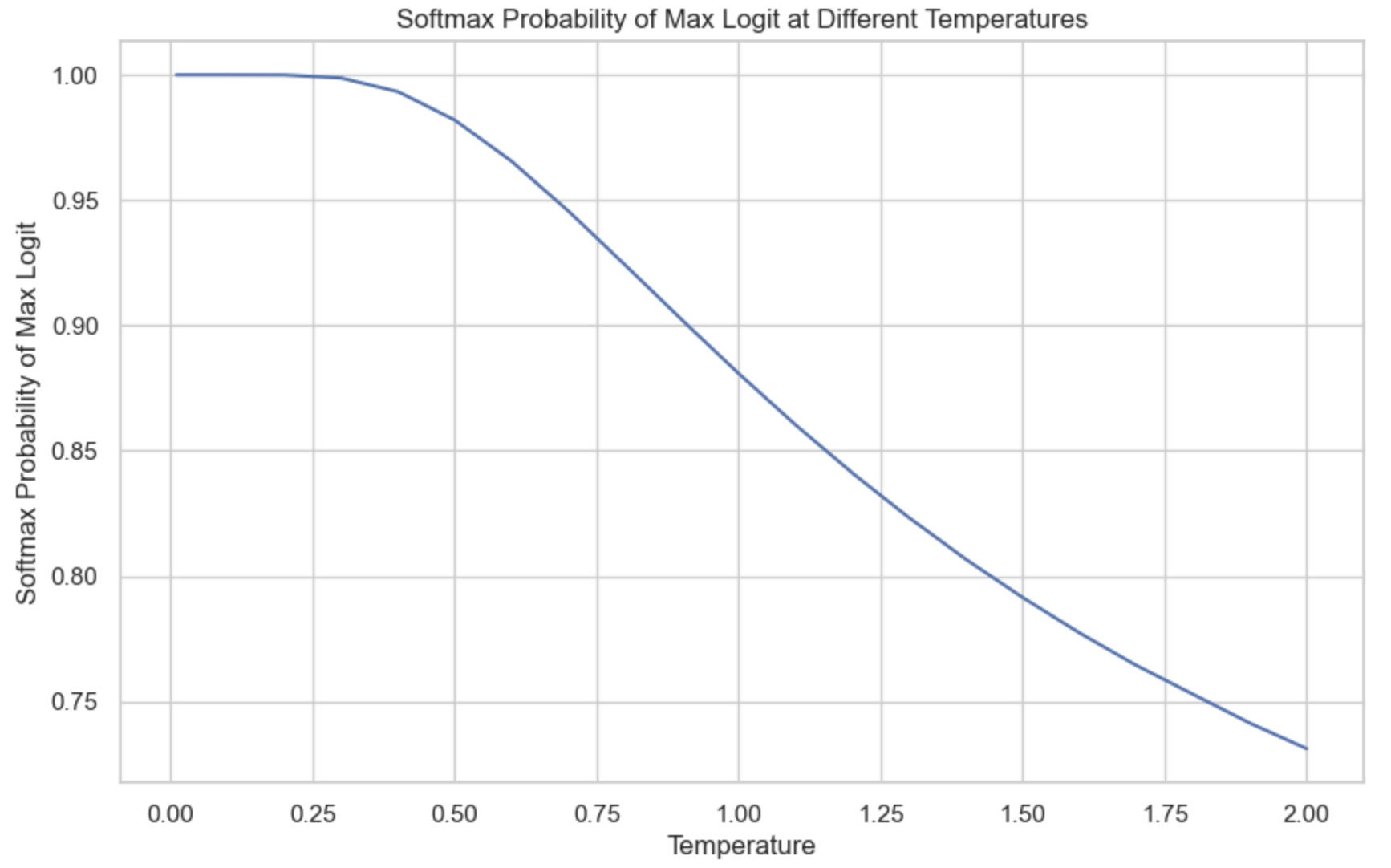
The higher the temperature, the less likely the model is going to pick the most obvious value (the value with the highest logit), making the model’s outputs more creative but potentially less coherent. The lower the temperature, the more likely the model is going to pick the most obvious value, making the model’s out more consistent but potentially more boring.
The graph below shows the softmax probability for token B at different temperatures. As the temperature gets closer to 0, the probability that the model picks token B becomes closer to 1. In our example, for temperature below 0.1, the model almost always outputs B. Model providers typically limit temperature to be between 0 and 2. If you own your model, you can use any non-negative temperature. A temperature of 0.7 is often recommended for creative use cases, as it balances creativity and determinism, but you should experiment and find the temperature that works best for you.
It’s common practice to set the temperature to 0 for the model’s outputs to be more consistent. Technically, temperature can never be 0 – logits can’t be divided by 0. In practice, when we set the temperature to 0, the model just picks the token with the value with the largest logit, e.g. performing an argmax, without doing the logit adjustment and softmax calculation.
A common debugging technique when working with an AI model is looking at the probabilities this model computes for given inputs. For example, if the probabilities look random, the model hasn’t learned much. OpenAI returns probabilities generated by their models as logprobs. Logprobs, short for log probabilities, are probabilities in the log scale. Log scale is preferred when working with a neural network’s probabilities because it helps reduce the underflow problem. A language model can work with a vocabulary size of 100,000, which means the probabilities for many of the tokens can be too small to be represented by a machine. The small numbers might be rounded down to 0. Log scale helps reduce this problem.
Top-k
Top-k is a sampling strategy to reduce the computation workload without sacrificing too much of the model’s response diversity. Recall that to compute the probability distribution over all possible values, a softmax layer is used. Softmax requires two passes over all possible values: one to perform the exponential sum \(\sum_j e^{x_j}\) and one to perform \(\frac{e^{x_i}}{\sum_j e^{x_j}}\) for each value. For a language model with a large vocabulary, this process is computationally expensive.
To avoid this problem, after the model has computed the logits, we pick the top k logits and perform softmax over these top k logits only. Depending on how diverse you want your application to be, k can be anywhere from 50 to 500, much smaller than a model’s vocabulary size. The model then samples from these top values. A smaller k value makes the text more predictable but less interesting, as the model is limited to a smaller set of likely words.
Top-p
In top-k sampling, the number of values considered is fixed to k. However, this number should change depending on the situation. For example, given the prompt Do you like music? Answer with only yes or no., the number of values considered should be two: yes and no. Given the prompt What's the meaning of life?, the number of values considered should be much larger.
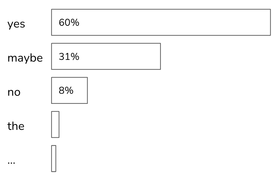
Top-p, also known as nucleus sampling, allows for a more dynamic selection of values to be sampled from. In top-p sampling, the model sums the probabilities of the most likely next values in descending order and stops when the sum reaches p. Only the values within this cumulative probability are considered. Common values for top-p (nucleus) sampling in language models typically range from 0.9 to 0.95. A top-p value of 0.9, for example, means that the model will consider the smallest set of values whose cumulative probability exceeds 90%.
Let’s say the probabilities of all tokens are as shown in the image below. If top_p = 90%, only yes and maybe will be considered, as their cumulative probability is greater than 90%. If top_p = 99%, then yes, maybe, and no are considered.
Unlike top-k, top-p doesn’t necessarily reduce the softmax computation load. Its benefit is that because it focuses on only the set of most relevant values for each context, it allows outputs to be more contextually appropriate. In theory, there doesn’t seem to be a lot of benefits to top-p sampling. However, in practice, top-p has proven to work well, causing its popularity to rise.
Stopping condition
An autoregressive language model generates sequences of tokens by generating one token after another. A long output sequence takes more time, costs more compute (money), and can sometimes be annoying to users. We might want to set a condition for the model to stop the sequence.
One easy method is to ask models to stop generating after a fixed number of tokens. The downside is that the output is likely to be cut off mid-sentence. Another method is to use stop tokens. For example, you can ask models to stop generating when it encounters “<EOS>”. Stopping conditions are helpful to keep the latency and cost down.
Test Time Compute
One simple way to improve a model’s performance is to generate multiple outputs and select the best one. This approach is called test time compute (or test time sampling).
You can either show users multiple outputs and let them choose the one that works best for them or devise a method to select the best one. If you want your model’s responses to be consistent, you want to keep all sampling variables fixed. However, if you want to generate multiple outputs and pick the best one, you don’t want to vary your sampling variables.
One selection method is to pick the output with the highest probability. A language model’s output is a sequence of tokens, each token has a probability computed by the model. The probability of an output is the product of the probabilities of all tokens in the output.
Consider the sequence of tokens [I, love, food] and:
- the probability for
Iis 0.2 - the probability for
lovegivenIis 0.1 - the probability for
foodgivenIandloveis 0.3
The sequence’s probability is then: 0.2 * 0.1 * 0.3 = 0.006.
Mathematically, this can be denoted as follows:
\[p(\text{I love food}) = p(\text{I}) \times p(\text{love}|\text{I}) \times p(\text{food}|\text{I, love})\]Remember that it’s easier to work with probabilities on a log scale. The logarithm of a product is equal to a sum of logarithms, so the logprob of a sequence of tokens is the sum of the logprob of all tokens in the sequence.
\[\text{logprob}(\text{I love food}) = \text{logprob}(\text{I}) + \text{logprob}(\text{love}|\text{I}) + \text{logprob}(\text{food}|\text{I, love})\]With summing, longer sequences are likely to have to lower total logprob (log(1) = 0, and log of all positive values less than 1 is negative). To avoid biasing towards short sequences, we use the average logprob by dividing the sum by its sequence length. After sampling multiple outputs, we pick the one with the highest average logprob. As of writing, this is what OpenAI API uses. You can set the parameter best_of to a specific value, say 10, to ask OpenAI models to return the output with the highest average logprob out of 10 different outputs.
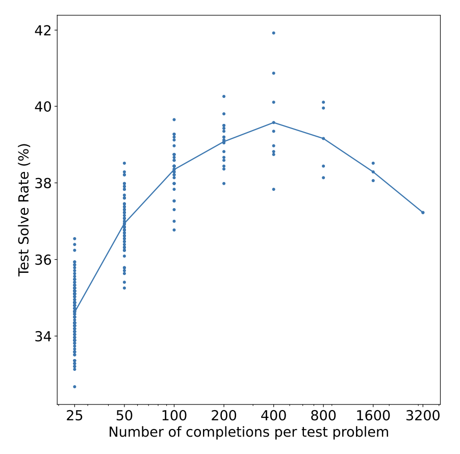
Another method is to use a reward model to score each output, as discussed in the previous section. Recall that both Stitch Fix and Grab pick the outputs given high scores by their reward models or verifiers. OpenAI also trained verifiers to help their models pick the best solutions to math problems (Cobbe et al., 2021). They found that sampling more outputs led to better performance, but only up to a certain point. In their experiment, this point is 400 outputs. Beyond this point, performance starts to decrease, as shown below. They hypothesized that as the number of sampled outputs increases, the chance of finding adversarial outputs that can fool the verifiers also increases. While this is an interesting experiment, I don’t believe anyone in production samples 400 different outputs for each input. The cost would be astronomical.
You can also choose heuristics based on the needs of your application. For example, if your application benefits from shorter responses, you can pick the shortest one. If your application is to convert from natural language to SQL queries, you can pick the valid SQL query that is the most efficient.
Sampling multiple outputs can be useful for tasks that expect exact answers. For example, given a math problem, the model can solve it multiple times and pick the most frequent answer as its final solution. Similarly, for a multiple-choice question, a model can pick the most frequently output option. This is what Google did when evaluating their model Gemini on MMLU, a benchmark of multiple-choice questions. They sampled 32 outputs for each question. While this helped Gemini achieve a high score on this benchmark, it’s unclear whether their model is better than another model that gets a lower score by only generating one output for each question.
The more fickle a model is, the more we can benefit from sampling multiple outputs. The optimal thing to do with a fickle model, however, is to swap it out for another. For one project, we used AI to extract certain information from an image of the product. We found that for the same image, our model could read the information only half of the time. For the other half, the model said that the image was too blurry or the text was too small to read. For each image, we queried the model at most three times, until it could extract the information.
While we can usually expect some model performance improvement by sampling multiple outputs, it’s expensive. On average, generating two outputs costs approximately twice as much as generating one.
Structured Outputs
Oftentimes, in production, we need models to generate text following certain formats. Having structured outputs is essential for the following two scenarios.
- Tasks whose outputs need to follow certain grammar. For example, for text-to-SQL or text-to-regex, outputs have to be valid SQL queries and regexes. For classification, outputs have to be valid classes.
- Tasks whose outputs are then parsed by downstream applications. For example, if you use an AI model to write product descriptions, you want to extract only the product descriptions without buffer texts like “Here’s the description” or “As a language model, I can’t …”. Ideally, for this scenario, models should generate structured outputs, such as JSON with specific keys, that can be parseable.
OpenAI was the first model provider to introduce JSON mode in their text generation API. Note that their JSON mode guarantees only that the outputs are valid JSON, not what’s inside the JSON. As of writing, OpenAI’s JSON mode doesn’t yet work for vision models, but I’m sure it’ll just be a matter of time.
The generated JSONs can also be truncated due to the model’s stopping condition, such as when it reaches the maximum output token length. If the max token length is set too short, the output JSONs can be truncated and hence not parseable. If it’s set too long, the model’s responses become both too slow and expensive.
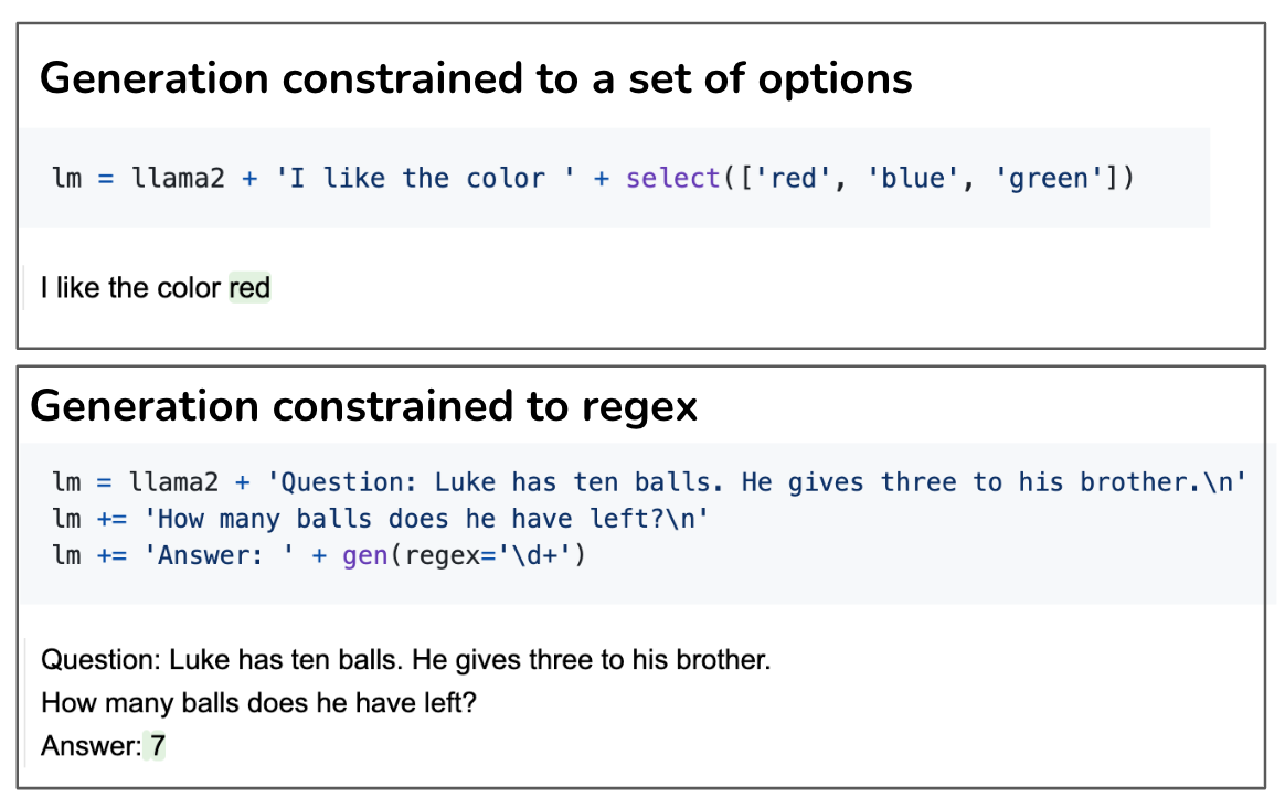
Independent tools like guidance and outlines let you structure the outputs of certain models. Here are two examples of using guidance to generate outputs constrained to a set of options and a regex.
How to generate structured outputs
You can guide a model to generate constrained outputs at different layers of the AI stack: during prompting, sampling, and finetuning. Prompting is currently the easiest but least effective method. You can instruct a model to output valid JSON following a specific schema. However, there’s no guarantee that the model will always follow this instruction.
Finetuning is currently the go-to approach to get models to generate outputs in the style and format that you want. You can do finetuning with or without changing the model’s architecture. For example, you can finetune a model on examples with the output format you want. While this still doesn’t guarantee the model will always output the expected format, this is much more reliable than prompting. It also has the added benefit of reducing inference costs, assuming that you no longer have to include instructions and examples of the desirable format in your prompt.
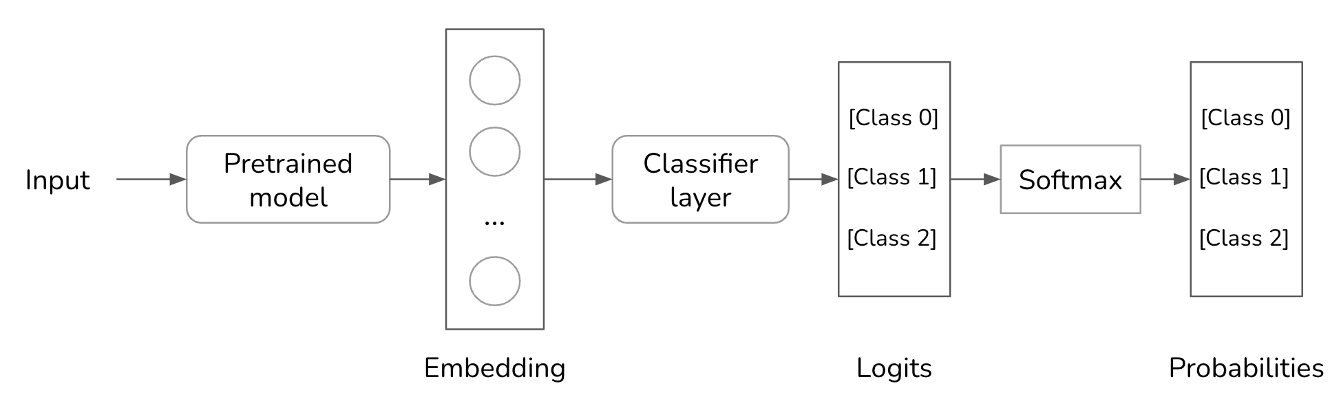
For certain tasks, you can guarantee the output format with finetuning by modifying the model’s architecture. For example, for classification, you can append a classifier head to the foundation model’s architecture to make sure that the model only outputs one of the pre-specified classes. During finetuing, you can retrain the entire architecture or only this classifier head.
Both sampling and finetuning techniques are needed because of the assumption that the model, by itself, isn’t capable of doing it. As models become more powerful, we can expect them to get better at following instructions. I suspect that in the future, it’ll be easier to get models to output exactly what we need with minimal prompting, and these techniques will become less important.
Constraint sampling
Constraint sampling is a technique used to guide the generation of text towards certain constraints. The simplest but expensive way to do so is to keep on generating outputs until you find one that fits your constraints, as discussed in the section Test Time Compute .
Constraint sampling can also be done during token sampling. I wasn’t able to find a lot of literature on how companies today are doing it. What’s written below is from my understanding, which can be wrong, so feedback and pointers are welcome!
At a high level, to generate a token, the model samples among values that meet the constraints. Recall that to generate a token, your model first outputs a logit vector, each logit corresponds to one possible value. With constrained sampling, we filter this logit vector to keep only the values that meet our constraints. Then we sample from these valid values.
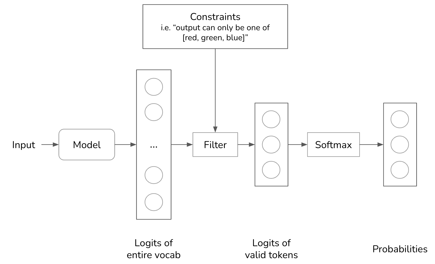
In the above example, the constraint is straightforward to filter for. However, in most cases, it’s not that straightforward. We need to have a grammar that specifies what is and isn’t allowed at each step. For example, JSON grammar dictates that after {, we can’t have another { unless it’s part of a string, as in {"key": ""}.
Building out that grammar and incorporating that grammar into the sampling process is non-trivial. We’d need a separate grammar for every output format we want: JSON, regex, CSV, etc. Some are against constrained sampling because they believe the resources needed for constrained sampling are better invested in training models to become better at following instructions.
Conclusion
I believe understanding how an AI model samples its outputs is essential for anyone who wishes to leverage AI to solve their problems. Probability is magical but can also be confusing. Writing this post has been a lot of fun as it gave me a chance to dig deeper into many concepts that I’ve been curious about for a long time.
As always, feedback is much appreciated. Thanks Han Lee and Luke Metz for graciously agreeing to be my first readers.