Data Distribution Shifts and Monitoring

Note: This note is a work-in-progress, created for the course CS 329S: Machine Learning Systems Design (Stanford, 2022).

• For the fully developed text, see the book Designing Machine Learning Systems (Chip Huyen, O’Reilly 2022).
• Slides (much shorter 😁).
• Original Google Docs version.

Let’s start the note with a story I was told by an executive that many readers might be able to relate to. About two years ago, his company hired a consulting firm to develop an ML model to help them predict how many of each grocery item they’d need next week, so they could restock the items accordingly. The consulting firm took six months to develop the model. When the consulting firm handed the model over, his company deployed it and was very happy with its performance. They could finally boast to their investors that they were an AI-powered company.

However, a year later, their numbers went down. The demand for some items was consistently being overestimated, which caused the extra items to expire. At the same time, the demand for some items was consistently being underestimated, leading to lost sales. Initially, his inventory team manually changed the model’s predictions to correct the patterns they noticed, but eventually, the model’s predictions had become so bad that they could no longer use it. They had three options: pay the same consulting firm an obscene amount of money to update the model, pay another consulting firm even more money because this firm would need time to get up to speed, or hire an in-house team to maintain the model onwards.

His company learned the hard way an important lesson that the rest of the industry is also discovering: deploying a model isn’t the end of the process. A model’s performance degrades over time in production. Once a model has been deployed, we still have to continually monitor its performance to detect issues as well as deploy updates to fix these issues.

---

Table of Contents
…. Natural Labels and Feedback Loop
…. Causes of ML System Failures
…….. Production Data Differing From Training Data
…….. Edge Cases
…….. Degenerate Feedback Loop
…. Data Distribution Shifts
…….. Types of Data Distribution Shifts
………… Covariate Shift
………… Label Shift
………… Concept Drift
…….. Handling Data Distribution Shifts
………… Detecting Data Distribution Shifts
………… Addressing Data Distribution Shifts
…. Monitoring and Observability
…….. ML-Specific Metrics
………… Monitoring Accuracy-Related Metrics
………… Monitoring Predictions
………… Monitoring Features
………… Monitoring Raw Inputs
…….. Monitoring Toolbox
………… Logs
………… Dashboards
………… Alerts
…….. Observability

---

Natural Labels and Feedback Loop

Tasks with natural ground truth labels are tasks where the model’s predictions can be automatically evaluated or partially evaluated by the system. An example is the model that estimates time of arrival on Google Maps. By the end of a trip, Google Maps knows how long the trip actually took, and thus can evaluate the accuracy of the predicted time of arrival.

Natural labels are ideal for evaluating a model’s performance. However, even if your task doesn’t inherently have natural labels, it’s possible to set up your system in a way that allows you to collect some feedback on your model. For example, if you’re building a translation system like Google Translate, you can have the option for the community to submit alternative translations for bad translations. Newsfeed ranking is not a task with inherent labels, but by adding the like button and other reactions to each newsfeed item, Facebook is able to collect feedback on their ranking algorithm.

For tasks with natural ground truth labels, the time it takes from when a prediction is served until when the feedback on it is provided is the feedback loop length.

Tasks with short feedback loops are tasks where ground truth labels are generally available within minutes. The canonical example of this type of task is recommender systems. The goal of a recommender system is to recommend users items they would like. Whether a user clicks on the recommended item or not can be seen as the feedback for that recommendation. A recommendation that gets clicked on can be presumed to be a good recommendation (i.e. the label is POSITIVE) and a recommendation that doesn’t get clicked on can be presumed to be bad (i.e. the label is NEGATIVE). Many tasks can be framed as recommendation tasks. For example, you can frame the task of predicting ads’ click-through rates as recommending the most relevant ads to users based on their activity histories and profiles.

However, not all recommender systems have short feedback loops. Depending on the nature of the item to be recommended, the delay until labels can be seconds to hours, and in some extreme cases, days or weeks. If the recommended items are subreddits to subscribe to on Reddit, people to follow on Twitter, videos to watch next on Tiktok, etc., the time between when the item is recommended until it’s clicked on, if it’s clicked on at all, is seconds. If you work with longer content types like blog posts or articles or YouTube videos, it can be minutes, even hours. However, if you build a system to recommend clothes for users like the one Stitch Fix has, you wouldn’t get feedback until users have received the items and tried them on, which could be weeks later.

Unless next to each recommended item, there’s a prompt that says: “Do you like this recommendation? Yes / No”, recommender systems don’t have explicit negative labels. Even if you add that prompt, there’s no guarantee that users will respond to it. Typically, a recommendation is presumed to be bad if there’s a lack of positive feedback. After a certain time window, if there is no click, the label is presumed to be negative. Choosing the right window length requires thorough consideration, as it involves the speed and accuracy tradeoff. A short window length means that you can capture labels faster, which allows you to use these labels for monitoring and continual learning. However, a short window length also means that you might prematurely label an item as no click before it’s being clicked on.

No matter how long you set your window length to be, there might still be premature negative labels. In early 2021, a study by the Ads team at Twitter found that even though the majority of clicks on ads happen within the first 5 minutes, some clicks happen hours after when the ad is shown. This means that this type of label tends to give an underestimate of the actual click-through rate. If you only record 1000 clicks, the actual number of clicks might be a bit over 1000 clicks.

For tasks with long feedback loops, natural labels might not arrive for weeks or even months. Fraud detection is an example of a task with long feedback loops. For a certain period of time after a transaction, users can dispute whether that transaction is fraudulent or not. For example, when a customer read their credit card’s statement and saw a transaction they didn’t recognize, they might dispute with their bank, giving the bank the feedback to label that transaction as fraudulent. A typical dispute window is a month to three months. After the dispute window has passed, if there’s no dispute from the user, you can presume the transaction to be legitimate.

Labels with long feedback loops are helpful for reporting a model’s performance on quarterly or yearly business reports. However, they are not very helpful if you want to detect issues with your models as soon as possible. If there’s a problem with your fraud detection model and it takes you months to catch, by the time the problem is fixed, all the fraudulent transactions your faulty model let through might have caused a small business to go bankrupt.

Causes of ML System Failures

Before we identify the cause of ML system failures, let’s briefly discuss what an ML system failure is. A failure happens when one or more expectations of the system is violated. In traditional software, we mostly care about a system’s operational expectations: whether the system executes its logics within the expected operational metrics such as the expected latency and throughput.

For an ML system, we care about both its operational metrics and its ML performance metrics. For example, consider an English-French machine translation system. Its operational expectation might be that given an English sentence, the system returns a French translation within a second latency. Its ML performance expectation is that the returned translation is an accurate translation of the original English sentence 99% of the time.

If you enter an English sentence into the system and don’t get back a translation, the first expectation is violated, so this is a system failure.

If you get back a translation that isn’t correct, it’s not necessarily a system failure because the accuracy expectation allows some margin of error. However, if you keep entering different English sentences into the system and keep getting back wrong translations, the second expectation is violated, which makes it a system failure.

Operational expectation violations are easier to detect, as they’re usually accompanied by an operational breakage such as a timeout, a 404 error on a webpage, an out of memory error, a segmentation fault, etc. However, ML performance expectation violations are harder to detect as it requires measuring and monitoring the performance of ML models in production. In the example of the English-French machine translation system above, detecting whether the returned translations are correct 99% of the time is difficult if we don’t know what the correct translations are supposed to be. There are countless examples of Google Translate’s painfully wrong translations being used by users because they aren’t aware that these are wrong translations. For this reason, we say that ML systems often fail silently.

To effectively detect and fix ML system failures in production, it’s useful to understand why a model, after proving to work well during development, would fail in production. We’ll examine two types of failures: Software system failures and ML-specific failures. Software system failures are failures that would have happened to non-ML systems. Here are some examples of software system failures.

1. Dependency failure: a software package or a codebase that your system depends on breaks, which leads your system to break. This failure mode is common when the dependency is maintained by a third party, and especially common if the third-party that maintains the dependency no longer exists¹.

2. Deployment failure: failures caused by deployment errors, such as when you accidentally deploy the binaries of an older version of your model instead of the current version, or when your systems don’t have the right permissions to read or write certain files.

3. Hardware failures: when the hardware that you use to deploy your model, such as CPUs or GPUs, doesn’t behave the way it should. For example, the CPUs you use might overheat and break down².

4. Downtime or crashing: if a component of your system runs from a server somewhere, such as AWS or a hosted service, and that server is down, your system will also be down.

Just because some failures are not specific to ML doesn’t mean it’s not important for ML engineers to understand. In 2020, Daniel Papasian and Todd Underwood, two ML engineers at Google, looked at 96 cases where a large ML pipeline at Google broke. They reviewed data from over the previous 15 years to determine the causes and found out that 60 out of these 96 failures happened due to causes not directly related to ML³. Most of the issues are related to distributed systems e.g. where the workflow scheduler or orchestrator makes a mistake, or related to the data pipeline e.g. where data from multiple sources is joined incorrectly or the wrong data structures are being used.

Addressing software system failures requires not ML skills, but traditional software engineering skills, and addressing them is beyond the scope of this class. Because of the importance of traditional software engineering skills in deploying ML systems, the majority of ML engineering is engineering, not ML⁴. For readers interested in learning how to make ML systems reliable from the software engineering perspective, I highly recommend the book Reliable Machine Learning, also published by O’Reilly with Todd Underwood as one of the authors.

A reason for the prevalence of software system failures is that because ML adoption in the industry is still nascent, tooling around ML production is limited and best practices are not yet well developed or standardized. However, as toolings and best practices for ML production mature, there are reasons to believe that the proportion of software system failures will decrease and the proportion of ML-specific failures will increase.

ML-specific failures are failures specific to ML systems. Examples include data collection and processing problems, poor hyperparameters, changes in the training pipeline not correctly replicated in the inference pipeline and vice versa, data distribution shifts that cause a model’s performance to deteriorate over time, edge cases, and degenerate feedback loop.

In this lecture, we’ll focus on addressing ML-specific failures. Even though they account for a small portion of failures, they can be more dangerous than non-ML failures as they’re hard to detect and fix, and can prevent ML systems from being used altogether. We’ve covered data problems, hyperparameter tuning, and the danger of having two separate pipelines for training and inference in previous lectures. In this lecture, we’ll discuss three new but very common problems that arise after a model has been deployed: changing data distribution, edge cases, and degenerate feedback loops.

Production Data Differing From Training Data

When we say that an ML model learns from the training data, it means that the model learns the underlying distribution of the training data with the goal of leveraging this learned distribution to generate accurate predictions for unseen data — data that it didn’t see during training. We’ll go into what this means mathematically in the Data Distribution Shifts section below. When the model is able to generate accurate predictions for unseen data, we say that this model “generalizes to unseen data.⁵” The test data that we use to evaluate a model during development is supposed to represent unseen data, and the model’s performance on the test data is supposed to give us an idea of how well the model will generalize.

One of the first things I learned in ML courses is that it’s essential for the training data and the unseen data to come from the same distribution. The assumption is that the unseen data comes from a stationary distribution that is the same as the training data distribution. If the unseen data comes from a different distribution, the model might not generalize well⁶.

This assumption is incorrect in most cases for two reasons. First, the underlying distribution of the real-world data is unlikely to be the same as the underlying distribution of the training data. Curating a training dataset that can accurately represent the data that a model will encounter in production turns out to be very difficult⁷. Real-world data is multi-faceted, and in many cases, virtually infinite, whereas training data is finite and constrained by the time, compute, and human resources available during the dataset creation and processing. There are many different selection and sampling biases that can happen and make real-world data diverge from training data. The divergence can be something as minor as real-world data using a different type of encoding of emojis. This type of divergence leads to a common failure mode known as the train-serving skew: a model that does great in development but performs poorly when deployed.

Second, the real world isn’t stationary. Things change. Data distributions shift. In 2019, when people searched for Wuhan, they likely wanted to get travel information, but since COVID-19, when people search for Wuhan, they likely want to know about the place where COVID-19 originated. Another common failure mode is that a model does great when first deployed, but its performance degrades over time as the data distribution changes. This failure mode needs to be continually monitored and detected for as long as a model remains in production.

When I use COVID-19 as an example that causes data shifts, some people have the impression that data shifts only happen because of unusual events, which implies they don’t happen often. Data shifts happen all the time, suddenly, gradually, or seasonally. They can happen suddenly because of a specific event, such as when your existing competitors change their pricing policies and you have to update your price predictions in response, or when you launch your product in a new region, or when a celebrity mentions your product which causes a surge in new users, and so on. They can happen gradually because social norms, cultures, languages, trends, industries, and more just change over time. They can also happen due to seasonal variations, such as people might be more likely to request rideshares in the winter when it’s cold and snowy than in the spring.

When talking about data shifts, many people imagine that they are due to external changes, such as natural disasters, holiday seasons, or user behaviors. But in reality, due to the complexity of ML systems and the poor practices in deploying them, a large percentage of what might look like data shifts on monitoring dashboards are caused by internal errors⁸, such as bugs in the data pipeline, missing values incorrectly filled in, inconsistencies between the features extracted during training and inference, features standardized using statistics from the wrong subset of data, wrong model version, or bugs in the app interface that forces users to change their behaviors.

Since this is an error mode that affects almost all ML models, we’ll cover this in detail in the section Data Distribution Shifts.

Edge Cases

Imagine there existed a self-driving car that can drive you safely 99.99% of the time, but the other 0.01% of the time, it might get into a catastrophic accident that can leave you permanently injured or even dead⁹. Would you use that car?

If you’re tempted to say no, you’re not alone. An ML model that performs well on most cases but fails on a small number of cases might not be usable if these failures cause catastrophic consequences. For this reason, major self-driving car companies are focusing on making their systems work on edge cases¹⁰¹¹¹².

Edge cases are the data samples so extreme that they cause the model to make catastrophic mistakes. Even though edge cases generally refer to data samples drawn from the same distribution, if there is a sudden increase in the number of data samples in which your model doesn’t perform well on, it could be an indication that the underlying data distribution has shifted.

Autonomous vehicles are often used to illustrate how edge cases can prevent an ML system from being deployed. But this is also true for any safety-critical application such as medical diagnosis, traffic control, eDiscovery¹³, etc. It can also be true for non-safety-critical applications. Imagine a customer service chatbot that gives reasonable responses to most of the requests, but sometimes, it spits out outrageously racist or sexist content. This chatbot will be a brand risk for any company that wants to use it, thus rendering it unusable.

Edge cases and outliers

You might wonder about the differences between an outlier and an edge case. The definition of what makes an edge case varies by discipline. In ML, because of its recent adoption in production, edge cases are still being discovered, which makes their definition contentious.

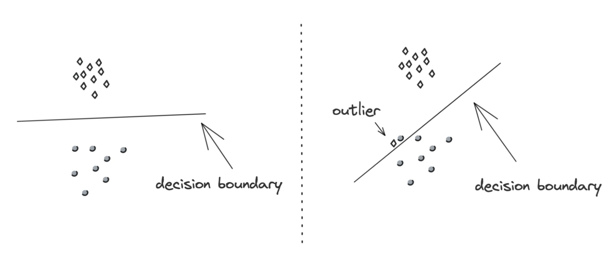
In this lecture, outliers refer to data: an example that differs significantly from other examples. Edge cases refer to performance: an example where a model performs significantly worse than other examples. An outlier can cause a model to perform unusually poorly, which makes it an edge case. However, not all outliers are edge cases. For example, a person jay-walking on a highway is an outlier, but it’s not an edge case if your self-driving car can accurately detect that person and decide on a motion response appropriately.

During model development, outliers can negatively affect your model’s performance. In many cases, it might be beneficial to remove outliers as it helps your model to learn better decision boundaries and generalize better to unseen data. However, during inference, you don’t usually have the option to remove or ignore the queries that differ significantly from other queries. You can choose to transform it — for example, when you enter “mechin learnin” into Google search, Google might ask if you mean “machine learning”. But most likely, you’ll want to develop a model so that it can perform well even on unexpected inputs.

The image on the left shows the decision boundary when there’s no outlier. The image on the right shows the decision boundary when there’s one outlier, which is very different from the decision boundary in the first case, and probably less accurate.

Degenerate Feedback Loop

In the Natural Labels and Feedback Loop section earlier in this lecture, we discussed a feedback loop as the time it took from when a prediction is shown until the time feedback on the prediction is provided. The feedback can be used to extract natural labels to evaluate the model’s performance.

A degenerate feedback loop can happen when the predictions themselves influence the feedback, which is then used to extract labels to train the next iteration of the model. More formally, a degenerate feedback loop is created when a system’s outputs are used to create or process the same system’s inputs, which, in turn, influence the system’s future outputs. In ML, a system’s predictions can influence how users interact with the system, and because users’ interactions with the system are sometimes used as the inputs to the same system, degenerate feedback loops can occur and cause unintended consequences. Degenerate feedback loops are especially common in tasks with natural labels from users, such as recommender systems and ads click-through-rate prediction.

To make this concrete, imagine you build a system to recommend to users songs that they might like. The songs that are ranked high by the system are shown first to users. Because they are shown first, users click on them more, which makes the system more confident that these recommendations are good. In the beginning, the rankings of two songs A and B might be only marginally different, but because A was originally ranked a bit higher, A got clicked on more, which made the system rank A even higher. After a while, A’s ranking became much higher than B¹⁴. Degenerate feedback loops are one reason why popular movies, books, or songs keep getting more popular, which makes it hard for new items to break into popular lists. This type of scenario is incredibly common in production and it’s heavily researched. It goes by many different names, including “exposure bias”, “popularity bias”, “filter bubbles,” and sometimes “echo chambers.”

Here’s another example to drive the idea of degenerative feedback loops home. Imagine building a resume-screening model to predict whether someone with a certain resume is qualified for the job. The model finds feature X accurately predicts whether someone is qualified, so it recommends resumes with feature X. You can replace X with features like “went to Stanford”, “worked at Google”, or “identifies as male”. Recruiters only interview people whose resumes are recommended by the model, which means they only interview candidates with feature X, which means the company only hires candidates with feature X. This, in turn, makes the model put even more weight on feature X¹⁵. Having visibility into how your model makes predictions — such as, measuring the importance of each feature for the model — can help detect the bias towards feature X in this case.

Left unattended, degenerate feedback loops can cause your model to perform suboptimally at best. At worst, it can perpetuate and magnify biases embedded in data, such as biasing against candidates without feature X above.

Detecting degenerate feedback loops

If degenerate feedback loops are so bad, how do we know if a feedback loop in a system is degenerate? When a system is offline, degenerate feedback loops are difficult to detect. Degenerate loops result from user feedback, and a system won’t have users until it’s online (e.g. deployed to users).

For the task of recommendation systems, it’s possible to detect degenerate feedback loops by measuring the popularity diversity of a system’s outputs even when the system is offline. An item’s popularity can be measured based on how many times it has been interacted with (e.g. seen, liked, bought, etc.) in the past. The popularity of all the items will likely follow a long tail distribution: a small number of items are interacted with a lot while most items are rarely interacted with at all. Various metrics such as aggregate diversity and average coverage of long tail items proposed by Brynjolfsson et al. (2011), Fleder et al. (2009), and Abdollahpouri et al. (2019) can help you measure the diversity of the outputs of a recommendation system. Low scores mean that the outputs of your system are homogeneous, which might be caused by popularity bias.

In 2021, Chia et al. went a step further and proposed the measurement of hit rate against popularity. They first divided items into buckets based on their popularity — e.g. bucket 1 consists of items that have been interacted with less than 100 times, bucket 2 consists of items that have been interacted with more than 100 times but less than 1000 times, etc. Then they measured the prediction accuracy of a recommender system for each of these buckets. If a recommender system is much better at recommending popular items than recommending less popular items, it likely suffers from popularity bias¹⁶. Once your system is in production and you notice that its predictions become more homogeneous over time, it likely suffers from degenerate feedback loops.

Correcting degenerate feedback loops

Because degenerate feedback loops are a common problem, there are many proposed methods on how to correct them. In this lecture, we’ll discuss two methods. The first one is to use randomization, and the second one is to use positional features.

We’ve discussed that degenerate feedback loops can cause a system’s outputs to be more homogeneous over time. Introducing randomization in the predictions can reduce their homogeneity. In the case of recommender systems, instead of showing the users only the items that the system ranks highly for them, we show users random items and use their feedback to determine the true quality of these items. This is the approach that TikTok follows. Each new video is randomly assigned an initial pool of traffic (which can be up to hundreds of impressions). This pool of traffic is used to evaluate each video’s unbiased quality to determine whether it should be moved to a bigger pool of traffic or to be marked as irrelevant¹⁷.

Randomization has been shown to improve diversity but at the cost of user experience¹⁸. Showing our users completely random items might cause users to lose interest in our product. An intelligent exploration strategy, such as contextual bandits, can help increase item diversity with acceptable prediction accuracy loss. Schnabel et al. uses a small amount of randomization and causal inference techniques to estimate the unbiased value of each song. They were able to show that this algorithm was able to correct a recommendation system to make recommendations fair to creators.

We’ve also discussed that degenerate feedback loops are caused by users’ feedback on predictions, and users’ feedback on a prediction is biased based on where it is shown. Consider the recommender system example above where each time you recommend 5 songs to users. You realize that the top recommended song is much more likely to be clicked on compared to the other 4 songs. You are unsure whether your model is exceptionally good at picking the top song, or whether users click on any song as long as it’s recommended on top.

If the position in which a prediction is shown affects its feedback in any way, you might want to encode the position information using positional features. Positional features can be numerical (e.g. positions are 1, 2, 3,..) or boolean (e.g. whether a prediction is shown in the first position or not). Note that “positional features” are different from “positional embeddings” mentioned in a previous lecture.

Here is a naive example to show how to use positional features. During training, you add “whether a song is recommended first” as a feature to your training data, as shown in Table 7-1. This feature allows your model to learn how much being a top recommendation influences how likely a song is clicked on.

Adding positional features to your training data to mitigate degenerate feedback loops.

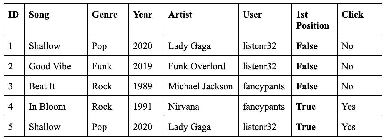
During inference, you want to predict whether a user will click on a song regardless of where the song is recommended, so you might want to set the 1st Position feature to be False. Then you look at the model’s predictions for various songs for each user and can choose the order in which to show each song.

This is a naive example because doing this alone might not be enough to combat degenerate feedback loops. A more sophisticated approach would be to use two different models. The first model predicts the probability that the user will see and consider a recommendation taking into account the position of that recommendation. The second model then predicts the probability that the user will click on the item given that they saw and considered it. The second model doesn’t concern positions at all.

Data Distribution Shifts

In the previous section, we’ve discussed common causes for ML system failures. In this section, we’ll zero in onto one especially sticky cause of failures: data distribution shifts, or data shifts for short. Data distribution shift refers to the phenomenon in supervised learning when the data a model works with changes over time, which causes this model’s predictions to become less accurate as time passes. The distribution of the data the model is trained on is called the source distribution. The distribution of the data the model runs inference on is called the target distribution.

Even though discussions around data distribution shift have only become common in recent years with the growing adoption of ML in the industry, data distribution shift in systems that learned from data has been studied as early as in 1986¹⁹. There’s also a book on dataset distribution shifts by Quiñonero-Candela et al. published by MIT Press in 2008.

Types of Data Distribution Shifts

While data distribution shift is often used interchangeably with concept drift and covariate shift and occasionally label shift, these are three distinct subtypes of data shift. To understand what they mean, we first need to define a couple of mathematical notations.

Let’s call the inputs to a model X and its outputs Y. We know that in supervised learning, the training data can be viewed as a set of samples from the joint distribution P(X, Y) and then ML usually models P(Y|X). This joint distribution P(X, Y) can be decomposed in two ways:

1. P(X, Y) = P(Y|X)P(X)
2. P(X, Y) = P(X|Y)P(Y)

P(Y|X) denotes the conditional probability of an output given an input — for example, the probability of an email being spam given the content of the email. P(X) denotes the probability density of the input. P(Y) denotes the probability density of the output. Label shift, covariate shift, and concept drift are defined as follows.

1. Covariate shift is when P(X) changes, but P(Y|X) remains the same. This refers to the first decomposition of the joint distribution.
2. Label shift is when P(Y) changes, but P(X|Y) remains the same. This refers to the second decomposition of the joint distribution.
3. Concept drift is when P(Y|X) changes, but P(X) remains the same. This refers to the first decomposition of the joint distribution²⁰.

If you find this confusing, don’t panic. We’ll go over examples in the following section to illustrate their differences.

Covariate Shift

Covariate shift is one of the most widely studied forms of data distribution shift²¹. In statistics, a covariate is an independent variable that can influence the outcome of a given statistical trial, but which is not of direct interest. Consider that you are running an experiment to determine how locations affect the housing prices. The housing price variable is your direct interest, but you know the square footage affects the price, so the square footage is a covariate. In supervised ML, the label is the variable of direct interest, and the input features are covariate variables.

Mathematically, covariate shift is when P(X) changes, but P(Y|X) remains the same, which means that the distribution of the input changes, but the conditional probability of a label given an input remains the same.

To make this concrete, consider the task of detecting breast cancer. You know that the risk of breast cancer is higher for women over the age of 40²², so you have a variable “age” as your input. You might have more women over the age of 40 in your training data than in your inference data, so the input distributions differ for your training and inference data. However, for an example with a given age, such as above 40, the probability that this example has breast cancer is constant. So P(Y|X), the probability of having breast cancer given age over 40, is the same.

During model development, covariate shifts can happen because of biases during the data selection process, which could result from the difficulty in collecting examples for certain classes. For example, suppose that to study breast cancer, you get data from a clinic where women go in to test for breast cancer. Because people over 40 are encouraged by their doctors to get checkups, your data is dominated by women over 40. For this reason, covariate shift is closely related to the sample selection bias problem²³.

Covariate shifts can also happen because the training data is artificially altered to make it easier for your model to learn. It’s hard for ML models to learn from imbalanced datasets, so you might want to collect more samples of the rare classes or oversample your data on the rare classes to make it easier for your model to learn the rare classes.

Covariate shift can also be caused by the model’s learning process, especially through active learning. In a previous lecture, we defined active learning as follows: instead of randomly selecting samples to train a model on, we use samples most helpful to that model according to some heuristics. This means that the training input distribution is altered by the learning process to differ from the real-world input distribution, and covariate shifts are a by-product²⁴.

In production, covariate shift usually happens because of major changes in the environment or in the way your application is used. Imagine you have a model to predict how likely a free user will convert to a paid user. The income level of the user is a feature. Your company’s marketing department recently launched a campaign that attracts users from a demographic more affluent than your current demographic. The input distribution into your model has changed, but the probability that a user with a given income level will convert remains the same.

Or consider you want to build a model to detect whether someone has COVID-19 from the sound of their coughs. To train your model, you use recordings collected from the hospitals. These recordings were recorded in quiet rooms with consistent starting times. However, when you deploy the model as a mobile application where users can cough directly into their phone microphones, the recordings will be very different — they might start several seconds before a cough or they might not start until the middle of coughing. They might also contain a wide variety of background noise. Your model’s performance on phone recordings won’t be very good.

If you know in advance how the real-world input distribution will differ from your training input distribution, you can leverage techniques such as importance weighting to train your model to work for the real world data. Importance weighting consists of two steps: estimate the density ratio between the real-world input distribution and the training input distribution, then weight the training data according to this ratio, and train an ML model on this weighted data²⁵²⁶.

However, because we don’t know in advance how the distribution will change in the real-world, it’s very difficult to preemptively train your models to make them robust to new, unknown distributions. There has been research that attempts to help models learn representations of latent variables that are invariant across data distributions, but I’m not aware of their adoption in the industry.

Label Shift

Label shift, also known as prior shift, prior probability shift or target shift, is when P(Y) changes but P(X|Y) remains the same. You can think of this as the case when the output distribution changes but for a given output, the input distribution stays the same.

Remember that covariate shift is when the input distribution changes. When the input distribution changes, the output distribution also changes, resulting in both covariate shift and label shift happening at the same time. Consider the breast cancer example for covariate shift above. Because there are more women over 40 in our training data than in our inference data, the percentage of POSITIVE labels is higher during training. However, if you randomly select person A with breast cancer from your training data and person B with breast cancer from your inference data, A and B have the same probability of being over 40. This means that P(X|Y), or probability of age over 40 given having breast cancer, is the same. So this is also a case of label shift.

However, not all covariate shifts result in label shifts. It’s a subtle point, so we’ll consider another example. Imagine that there is now a preventive drug that every woman takes that helps reduce their chance of getting breast cancer. The probability P(Y|X) reduces for women of all ages, so it’s no longer a case of covariate shift. However, given a person with breast cancer, the age distribution remains the same, so this is still a case of label shift.

Because label shift is closely related to covariate shift, methods for detecting and adapting models to label shifts are similar to covariate shift adaptation methods. We’ll discuss them more in the Handling Data Shifts section below.

Concept Drift

Concept drift, also known as posterior shift, is when the input distribution remains the same but the conditional distribution of the output given an input changes. You can think of this as “same input, different output”. Consider you’re in charge of a model that predicts the price of a house based on its features. Before COVID-19, a 3 bedroom apartment in San Francisco could cost $2,000,000. However, at the beginning of COVID-19, many people left San Francisco, so the same house would cost only $1,500,000. So even though the distribution of house features remains the same, the conditional distribution of the price of a house given its features has changed.

In many cases, concept drifts are cyclic or seasonal. For example, rideshare’s prices will fluctuate on weekdays versus weekends, and flight tickets rise during holiday seasons. Companies might have different models to deal with cyclic and seasonal drifts. For example, they might have one model to predict rideshare prices on weekdays and another model for weekends.

General Data Distribution Shifts

There are other types of changes in the real-world that, even though not well-studied in research, can still degrade your models’ performance.

One is feature change, such as when new features are added, older features are removed, or the set of all possible values of a feature changes²⁷. For example, your model was using years for the “age” feature, but now it uses months, so the range of this feature values has drifted. One time, our team realized that our model’s performance plummeted because a bug in our pipeline caused a feature to become NaNs.

Label schema change is when the set of possible values for Y change. With label shift, P(Y) changes but P(X|Y) remains the same. With label schema change, both P(Y) and P(X|Y) change. A schema describes the structure of the data, so the label schema of a task describes the structure of the labels of that task. For example, a dictionary that maps from a class to an integer value, such as {“POSITIVE”: 0, “NEGATIVE”: 1}, is a schema.

With regression tasks, label schema change could happen because of changes in the possible range of label values. Imagine you’re building a model to predict someone’s credit score. Originally, you used a credit score system that ranged from 300 to 850, but you switched to a new system that ranges from 250 to 900.

With classification tasks, label schema change could happen because you have new classes. For example, suppose you are building a model to diagnose diseases and there’s a new disease to diagnose. Classes can also become outdated or more fine-grained. Imagine that you’re in charge of a sentiment analysis model for tweets that mention your brand. Originally, your model predicted only 3 classes: POSITIVE, NEGATIVE, and NEUTRAL. However, your marketing department realized the most damaging tweets are the angry ones, so they wanted to break the NEGATIVE class into two classes: SAD and ANGRY. Instead of having three classes, your task now has four classes. When the number of classes changes, your model’s structure might change,²⁸ and you might need to both relabel your data and retrain your model from scratch. Label schema change is especially common with high-cardinality tasks — tasks with a high number of classes — such as product or documentation categorization.

There’s no rule that says that only one type of shift should happen at one time. A model might suffer from multiple types of drift, which makes handling them a lot more difficult.

Handling Data Distribution Shifts

How companies handle data shifts depends on how sophisticated their ML infrastructure setups are. At one end of the spectrum, we have companies that have just started with ML and are still working on getting ML models into production, so they might not have gotten to the point where data shifts are catastrophic to them. However, at some point in the future — maybe 3 months, maybe 6 months — they might realize that their initial deployed models have degraded to the point that they do more harm than good. They will then need to adapt their models to the shifted distributions or to replace them with other solutions.

At the same time, many companies assume that data shifts are inevitable, so they periodically retrain their models — once a quarter, once a month, once a week, or even once a day — regardless of the extent of the shift. How to determine the optimal frequency to retrain your models is an important decision that many companies still determine based on gut feelings instead of experimental data²⁹. We’ll discuss more about the retraining frequency in the lecture on Continual Learning.

Many companies want to handle data shifts in a more targeted way, which consists of two parts: first, detecting the shift and second, addressing the shift.

Detecting Data Distribution Shifts

Data distribution shifts are only a problem if they cause your model’s performance to degrade. So the first idea might be to monitor your model’s accuracy-related metrics³⁰ in production to see whether they have changed. “Change” here usually means “decrease”, but if my model’s accuracy suddenly goes up or fluctuates significantly for no reason that I’m aware of, I’d want to investigate.

Accuracy-related metrics work by comparing the model’s predictions to ground truth labels³¹. During model development, you have access to ground truth, but in production, you don’t always have access to ground truth, and even if you do, ground truth labels will be delayed, as discussed in the section Natural Labels and Feedback Loop above. Having access to ground truth within a reasonable time window will vastly help with giving you visibility into your model’s performance.

When ground truth labels are unavailable or too delayed to be useful, we can monitor other distributions of interest instead. The distributions of interest are the input distribution P(X), the label distribution P(Y), and the conditional distributions P(X|Y) and P(Y|X).

While we don’t need to know the ground truth labels Y to monitor the input distribution, monitoring the label distribution and both of the conditional distributions require knowing Y. In research, there have been efforts to understand and detect label shifts without labels from the target distribution. One such effort is Black Box Shift Estimation by Lipton et al., 2018. However, in the industry, most drift detection methods focus on detecting changes in the input distribution, especially the distributions of features.

Statistical methods

In industry, a simple method many companies use to detect whether the two distributions are the same is to compare their statistics like mean, median, variance, quantiles, skewness, kurtosis, etc. For example, you can compute the median and variance of the values of a feature during inference and compare them to the metrics computed during training. As of October 2021, even TensorFlow Extended’s built-in data validation tools use only summary statistics to detect the skew between the training and serving data and shifts between different days of training data. This is a good start, but these metrics are far from sufficient³². Mean, median, and variance are only useful with the distributions for which the mean/median/variance are useful summaries. If those metrics differ significantly, the inference distribution might have shifted from the training distribution. However, if those metrics are similar, there’s no guarantee that there’s no shift.

A more sophisticated solution is to use a two-sample hypothesis test, shortened as two-sample test. It’s a test to determine whether the difference between two populations (two sets of data) is statistically significant. If the difference is statistically significant, then the probability that the difference is a random fluctuation due to sampling variability is very low, and therefore, the difference is caused by the fact that these two populations come from two distinct distributions. If you consider the data from yesterday to be the source population and the data from today to be the target population and they are statistically different, it’s likely that the underlying data distribution has shifted between yesterday and today.

A caveat is that just because the difference is statistically significant doesn’t mean that it is practically important. However, a good heuristic is that if you are able to detect the difference from a relatively small sample, then it is probably a serious difference. If it takes a huge sample, then it is probably not worth worrying about.

A basic two-sample test is the Kolmogorov–Smirnov test, also known as K-S or KS test³³. It’s a nonparametric statistical test, which means it doesn’t require any parameters of the underlying distribution to work. It doesn’t make any assumption about the underlying distribution, which means it can work for any distribution. However, one major drawback of the KS test is that it can only be used for one-dimensional data. If your model’s predictions and labels are one-dimensional (scalar numbers), then the KS test is useful to detect label or prediction shifts. However, it won’t work for high-dimensional data, and features are usually high-dimensional³⁴. K-S tests can also be expensive and produce too many false positive alerts³⁵.

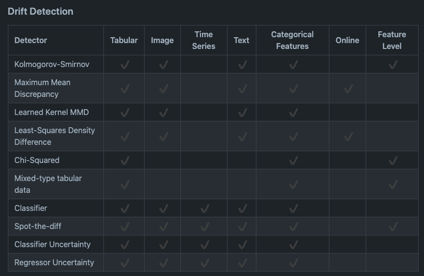
Another test is Least-Squares Density Difference, an algorithm that is based on the least squares density-difference estimation method³⁶. There is also MMD, Maximum Mean Discrepancy, (Gretton et al. 2012) a kernel-based technique for multivariate two-sample testing and its variant Learned Kernel MMD (Liu et al., 2020). MMD is popular in research, but as of writing this note, I’m not aware of any company that is using it in the industry. alibi-detect is a great open-source package with the implementations of many drift detection algorithms.

Some drift detection algorithms implemented by alibi-detect. Image screenshotted from its GitHub repository.

Because two-sample tests often work better on low-dimensional data than on high-dimensional data, it’s highly recommended that you reduce the dimensionality of your data before performing a two-sample test on them³⁷.

Time scale windows for detecting shifts

Not all types of shifts are equal — some are harder to detect than others. For example, shifts happen at different rates, and abrupt changes are easier to detect than slow, gradual changes³⁸. Shifts can also happen across two dimensions: spatial or temporal. Spatial shifts are shifts that happen across access points, such as your application gets a new group of users or your application is now served on a different type of device. Temporal shifts are shifts that happen over time. To detect temporal shifts, a common approach is to treat input data to ML applications as time series data³⁹.

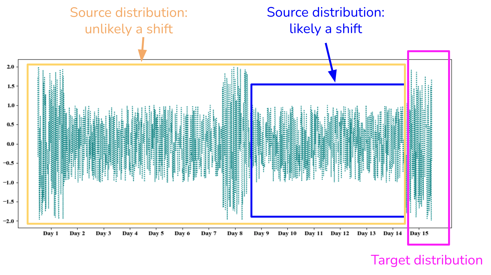
When dealing with temporal shifts, the time scale window of the data we look at affects the shifts we can detect. If your data has a weekly cycle, then a time scale of less than a week won’t detect the cycle. Consider the data in the figure below. If we use data from day 9 to day 14 as the source distribution, then day 15 looks like a shift. However, if we use data from day 1 to day 14 as the source distribution, then all data points from day 15 are likely being generated by that same distribution. As illustrated by this example, detecting temporal shifts is hard when shifts are confounded by seasonal variation.

Whether a distribution has drifted over time depends on the time scale window specified. If we use data from day 9 to day 14 as the base distribution, then day 15 looks like a drift. However, if we use data from day 1 to day 14 as the base distribution, then all data points from day 15 are likely being generated by that same distribution.

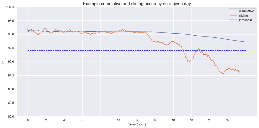
When computing running statistics over time, it’s important to differentiate between cumulative and sliding statistics. Sliding statistics are computed within a single time scale window, e.g. an hour. Cumulative statistics are continually updated with more data. This means for each the beginning of each time scale window, the sliding accuracy is reset, whereas the cumulative sliding accuracy is not. Because cumulative statistics contain information from previous time windows, they might obscure what happens in a specific time window. This is an example of how cumulative accuracy can hide the sudden dip in accuracy between the hour 16 and 18. This image is based on an example from MadeWithML.

Cumulative accuracy hides the sudden dip in accuracy between the hour 16 and 18.

Working with data in the temporal space makes things so much more complicated, requiring knowledge of time series analysis techniques such as time series decompositions that are beyond the scope of this class. For readers interested in time series decomposition, here’s a great case study by Lyft engineering on how they decompose their time series data to deal with the seasonality of the market.

As of today, many companies use the distribution of the training data as the base distribution and monitor the production data distribution at a certain granularity level, such as hourly and daily⁴⁰. The shorter your time scale window, the faster you’ll be able to detect changes in your data distribution. However, too short a time scale window can lead to false alarms of shifts, like the example above.

Some platforms, especially those dealing with real-time data analytics such as monitoring, provide a merge operation that allows merging statistics from shorter time scale windows to create statistics for larger time scale windows. For example, you can compute the data statistics you care about hourly, then merge these hourly statistics chunks into daily views.

More advanced monitoring platforms even attempt a root cause analysis (RCA) feature that automatically analyzes statistics across various time window sizes to detect exactly the time window where a change in data happened⁴¹.

Addressing Data Distribution Shifts

To make a model work with a new distribution in production, there are three main approaches. The first is the approach that currently dominates research: train models using massive datasets. The hope here is that if the training dataset is large enough, the model will be able to learn such a comprehensive distribution that whatever data points the model will encounter in production will likely come from this distribution.

The second approach, less popular in research, is to adapt a trained model to a target distribution without requiring new labels. Zhang et al. (2013) used causal interpretations together with kernel embedding of conditional and marginal distributions to correct models’ predictions for both covariate shifts and label shifts without using labels from the target distribution. Similarly, Zhao et al. (2020) proposed domain-invariant representation learning: an unsupervised domain adaptation technique that can learn data representations invariant to changing distributions. However, this area of research is heavily underexplored and hasn’t found wide adoption in industry⁴².

The third approach is what is usually done in the industry today: retrain your model using the labeled data from the target distribution. However, retraining your model is not so straightforward. Retraining can mean retraining your model from scratch on both the old and new data or continuing training the existing model on new data. The latter approach is also called fine-tuning.

If you want to fine-tune your model, the question might be what data to use: data from the last hour, last 24 hours, last week, or last 6 months. A common practice is to fine-tune your model from the point when data has started to drift. Another is to fine-tune your model using the data gathered from the last fine-tuning. You might need to run experiments to figure out which retraining solution works best for you⁴³.

Fine-tuning on only new data is obviously preferred because it requires less computing resources and runs faster than retraining a model from scratch on both the old and new data. However, depending on their setups, many companies find that fine-tuning doesn’t give their models good-enough performance, and therefore have to fall back to retraining from scratch.

In this lecture, we use “retraining” to refer to both training from scratch and fine-tuning.

Readers familiar with data shift literature might often see data shifts mentioned along with domain adaptation and transfer learning. If you consider a distribution to be a domain, then the question of how to adapt your model to new distributions is similar to the question of how to adapt your model to different domains.

Similarly, if you consider learning a joint distribution P(X, Y) as a task, then adapting a model trained on one joint distribution for another joint distribution can be framed as a form of transfer learning. Transfer learning refers to the family of methods where a model developed for a task is reused as the starting point for a model on a second task. The difference is that with transfer learning, you don’t retrain the base model from scratch for the second task. However, to adapt your model to a new distribution, you might need to retrain your model from scratch.

Addressing data distribution shifts doesn’t have to start after the shifts have happened. It’s possible to design your system to make it more robust to shifts. A system uses multiple features, and different features shift at different rates. Consider that you’re building a model to predict whether a user will download an app. You might be tempted to use that app’s ranking in the app store as a feature since higher ranking apps tend to be downloaded more. However, app ranking changes very quickly. You might want to instead bucket each app’s ranking into general categories such as top 10, between 11 - 100, between 101 - 1000, between 1001 - 10,000, and so on. At the same time, an app’s categories might change a lot less frequently, but might have less power to predict whether a user will download that app. When choosing features for your models, you might want to consider the trade-off between the performance and the stability of a feature: a feature might be really good for accuracy but deteriorate quickly, forcing you to train your model more often.

You might also want to design your system to make it easier for it to adapt to shifts. For example, housing prices might change a lot faster in major cities like San Francisco than in rural Arizona, so a housing price prediction model serving rural Arizona might need to be updated less frequently than a model serving San Francisco. If you use the same model to serve both markets, you’ll have to use data from both markets to update your model at the rate demanded by San Francisco. However, if you use a separate model for each market, you can update each of them only when necessary.

Before we move on to the next lecture, I just want to reiterate that not all performance degradation of models in production requires ML solutions. Many ML failures today, not software system failures and ML-specific failures, are still caused by human errors. If your model failure is caused by human errors, you’d first need to find those errors to fix them. Detecting a data shift is hard, but determining what causes a shift can be even harder.

Monitoring and Observability

As the industry realized that many things can go wrong with an ML system, many companies started investing in monitoring and observability for their ML systems in production.

Monitoring and observability are sometimes used exchangeably, but they are different. Monitoring refers to the act of tracking, measuring, and logging different metrics that can help us determine when something goes wrong. Observability means setting up our system in a way that gives us visibility into our system to help us investigate what went wrong. The process of setting up our system in this way is also called “instrumentation”. Examples of instrumentation are adding timers to your functions, counting NaNs in your features, tracking how inputs are transformed through your systems, logging unusual events such as unusually long inputs, etc. Observability is part of monitoring. Without some level of observability, monitoring is impossible.

Monitoring is all about metrics. Because ML systems are software systems, the first class of metrics you’d need to monitor are the operational metrics. These metrics are designed to convey the health of your systems. They are generally divided into three levels: the network the system is run on, the machine the system is run on, and the application that the system runs. Examples of these metrics are latency, throughput, the number of prediction requests your model receives in the last minute, hour, day, the percentage of requests that return with a 2XX code, CPU/GPU utilization, memory utilization, etc. No matter how good your ML model is, if the system is down, you’re not going to benefit from it.

Let’s look at an example. One of the most important characteristics of a software system in production is availability — how often the system is available to offer reasonable performance to users. This characteristic is measured by uptime, the percentage of time a system is up. The conditions to determine whether a system is up are defined in the service level objectives (SLOs) or service level agreements (SLAs). For example, an SLA may specify that the service is considered to be up if it has a median latency of less than 200 ms and a 99th percentile under 2s.

Note: How important availability is to a system is a tradeoff decision. The CAP theorem states that any distributed data store can only provide two of the following three guarantees: Consistency, Availability, and Partition tolerance.

A service provider might offer an SLA that specifies their uptime guarantee, such as 99.99% of the time, and if this guarantee is not met, they’ll give their customers back money. For example, as of October 2021, AWS EC2 service offers a monthly uptime percentage of at least 99.99% (four nines), and if the monthly uptime percentage is lower than that, they’ll give you back a service credit towards future EC2 payments. 99.99% monthly uptime means the service is only allowed to be down a little over 4 minutes a month, and 99.999% means only 26 seconds a month!

However, for ML systems, the system health extends beyond the system uptime. If your ML system is up but its predictions are garbage, your users aren’t going to be happy. Another class of metrics you’d want to monitor are ML-specific metrics that tell you the health of your ML models.

ML-Specific Metrics

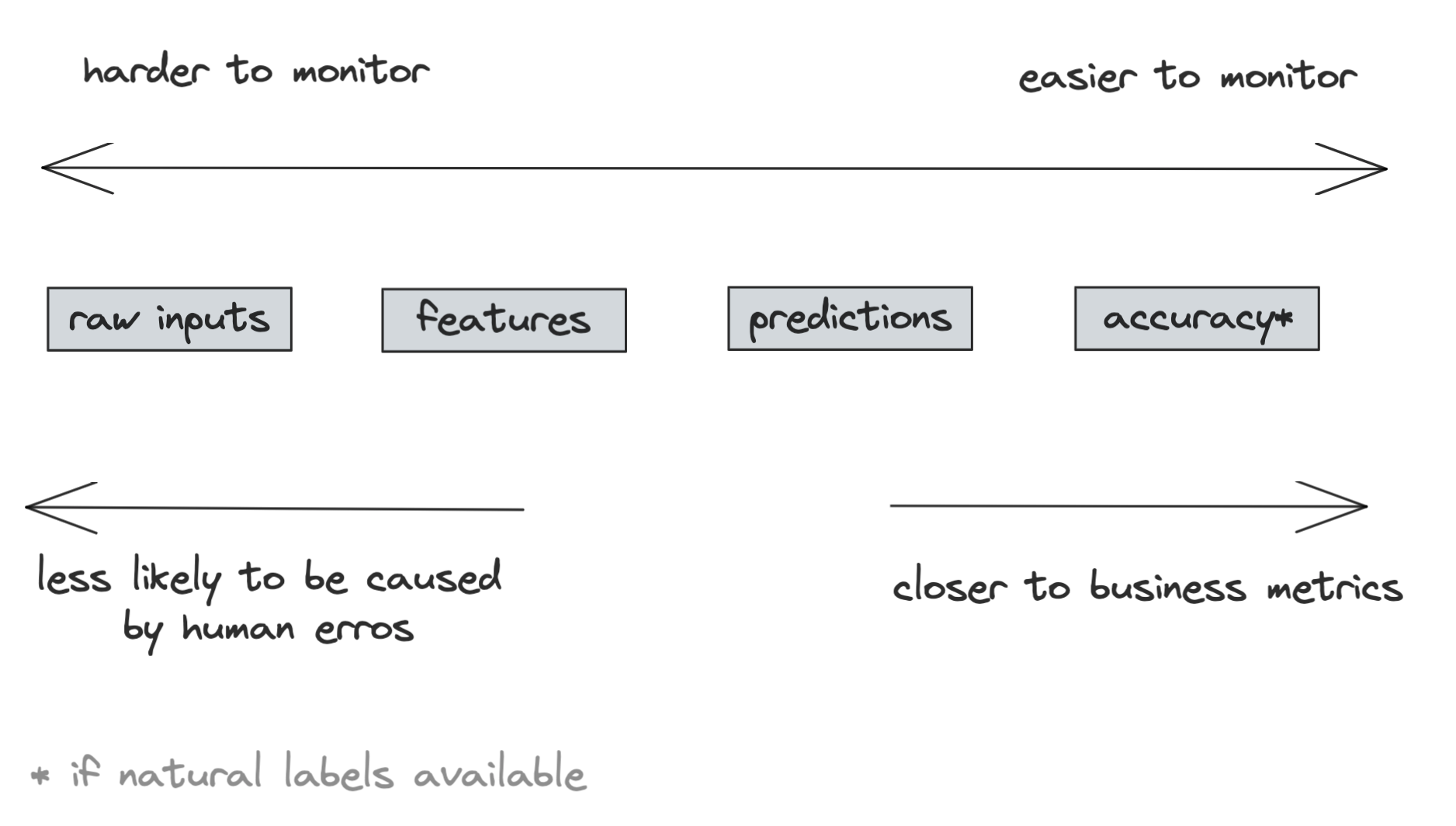
Within ML-specific metrics, there are generally four artifacts to monitor: model’s accuracy-related metrics, predictions, features, and raw inputs. These are artifacts generated at four different stages of an ML system pipeline. The deeper into the pipeline an artifact, the more transformations it has gone through, which makes a change in that artifact more likely to be caused by errors in one of those transformations. However, the more transformations an artifact has gone through, the more structured it’s become and the closer it is to the metrics you actually care about, which makes it easier to monitor. We’ll look at each of these artifacts in detail in the following sections.

The more transformations an artifact has gone through, the more likely that its changes are likely to be caused by errors in one of those transformations.

Monitoring Accuracy-Related Metrics

If your system receives any type of user feedback for the predictions it makes — click, hide, purchase, upvote, downvote, favorite, bookmark, share, etc. — you should definitely log and track it. Some feedback can be used to infer natural labels which can then be used to calculate your model’s accuracy-related metrics. Accuracy-related metrics are the most direct metrics to help you decide whether a model’s performance has degraded.

Even if the feedback can’t be used to infer natural labels directly, it can be used to detect changes in your ML model’s performance. For example, when you’re building a system to recommend to users what videos to watch next on YouTube, you want to track not only whether the users click on a recommended video (click-through rate), but also the duration of time users spend on that video and whether they complete watching it (completion rate). If over time, the click through rate remains the same but the completion rate drops, it might mean that your recommendation system is getting worse.

Monitoring Predictions

Prediction is the most common artifact to monitor. If it’s a regression task, each prediction is a continuous value (e.g. the predicted price of a house), and if it’s a classification task, each prediction is a discrete value corresponding to the predicted category. Because each prediction is usually just a number (low dimension), predictions are easy to visualize, and their summary statistics are straightforward to compute and interpret.

You can monitor predictions for distribution shifts. Because predictions are low dimensional, it’s also easier to compute two-sample tests to detect whether the prediction distribution has shifted. Prediction distribution shifts are also a proxy for input distribution shifts. Assuming that the function that maps from input to output doesn’t change — the weights and biases of your model haven’t changed — then a change in the prediction distribution generally indicates a change in the underlying input distribution.

You can also monitor predictions for anything odd happening to it, such as predicting an unusual amount of False in a row. There could be a long delay between predictions and ground truth labels. Changes in accuracy-related metrics might not become obvious for days or weeks, whereas a model predicting all False for 10 minutes can be detected immediately.

Monitoring Features

ML monitoring solutions in the industry focus on tracking changes in features, both the features that a model uses as inputs and the intermediate transformations from raw inputs into final features. Feature monitoring is appealing because compared to raw input data, features are well-structured following a predefined schema. The first step of feature monitoring is feature validation: ensuring that your features follow an expected schema. If these expectations are violated, there might be a shift in the underlying distribution. For example, here are some of the things you can check for a given feature:

• If the min, max, or median values of a feature are within an acceptable range
• If the values of a feature satisfy a regex format
• If all the values of a feature belong to a predefined set
• If the values of a feature are always greater than the values of another feature

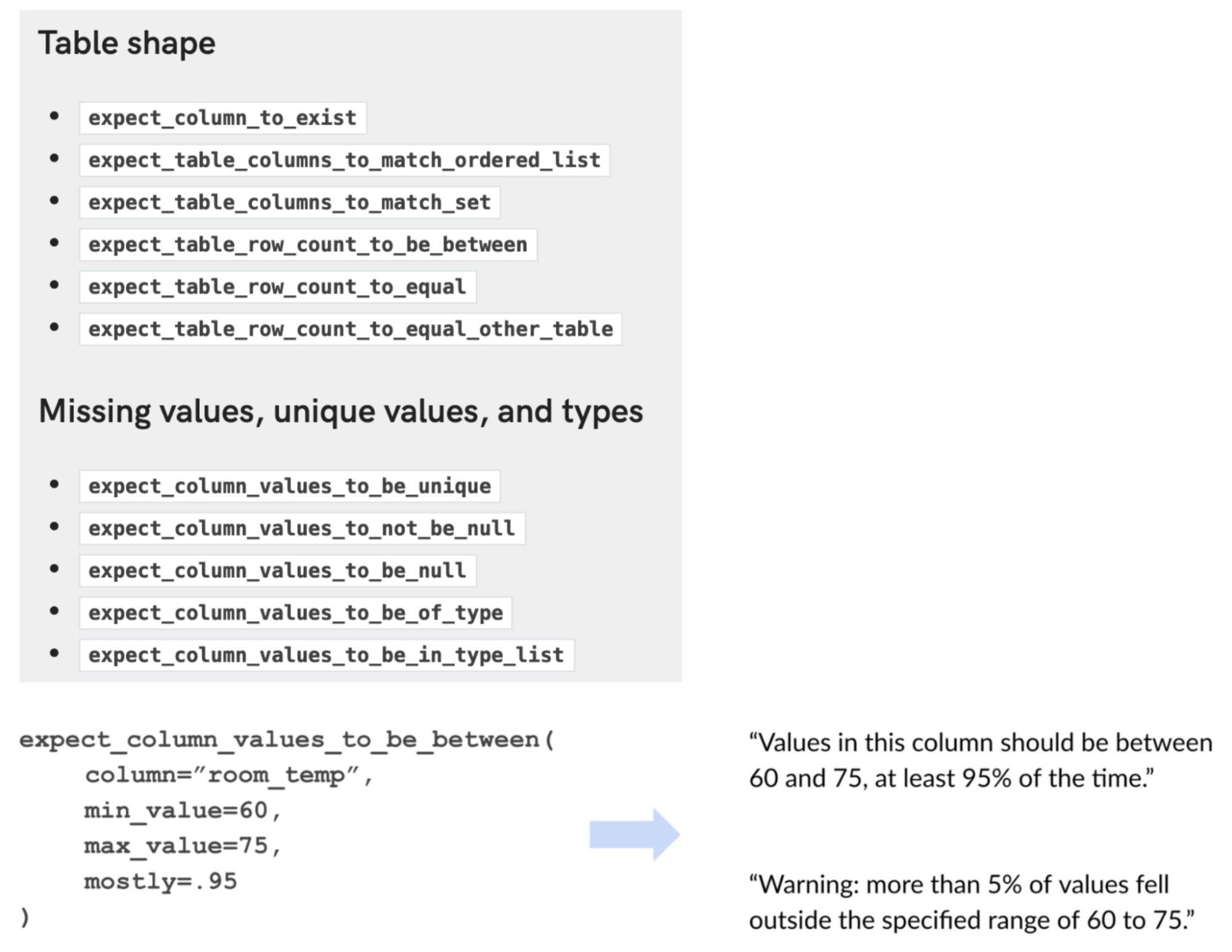
Because features are often organized into tables — each column representing a feature and each row representing a data sample — feature validation is also known as table testing or table validation. Some call them unit tests for data. There are many open source libraries that help you do basic feature validation, and the two most common are Great Expectations and Deequ, which is by AWS. This picture below shows some of the built-in feature validation functions by Great Expectations and an example of how to use them.

Some of the built-in feature validation functions by Great Expectations and an example of how to use them. Screenshotted from Great Expectations’ GitHub repository.

Beyond basic feature validation, you can also use two-sample tests to detect whether the underlying distribution of a feature or a set of features has shifted. Since a feature or a set features can be high-dimensional, you might need to reduce their dimension before performing the test on them, which can make the test less effective.

There are four major concerns when doing feature monitoring. First, a company might have hundreds of models in production, each model uses hundreds, if not thousands of features. Even something as simple as computing summary statistics for all these features every hour can be expensive, not only in terms of compute required but also memory used. Tracking too many metrics, i.e. constantly computing too many metrics, can also slow down your system, and increase both the latency that your users experience and the time it takes for you to detect anomalies in your system.

Second, while tracking features is useful for debugging purposes, it’s not very useful for detecting model performance degradation. In theory, a small distribution shift can cause catastrophic failure, but in practice, an individual feature’s minor changes might not harm the model’s performance at all. Feature distributions shift all the time, and most of these changes are benign⁴⁴. If you want to be alerted whenever a feature seems to have drifted, you might soon be overwhelmed by alerts and realize that most of these alerts are false positives. This can cause a phenomenon called “alert fatigue” where the monitoring team stops paying attention to the alerts because they are so frequent. The problem of feature monitoring becomes the problem of trying to decide which feature shifts are critical, which are not.

The third concern is that feature extraction is often done in multiple steps (such as filling missing values and standardization), using multiple libraries (such as Pandas, Spark), on multiple services (such as Kubernetes or Snowflake). You might have a relational database as an input to the feature extraction process and a NumPy array as the output. Even if you detect a harmful change in a feature, it might be impossible to detect whether this change is caused by a change in the underlying input distribution or whether it’s caused by an error in one of the multiple processing steps.

The fourth concern is that the schema that your features follow can change over time. If you don’t have a way to version your schemas and map each of your features to its expected schema, the cause of the reported alert might be due to the mismatched schema rather than a change in the data.

Monitoring Raw Inputs

What if we move the monitoring to one step earlier towards the raw inputs? The raw input data might not be easier to monitor, as they can come from multiple sources in different formats, following multiple structures. The way many ML workflows are set up today also makes it impossible for ML engineers to get direct access to raw input data, as the raw input data is often managed by a data platform team who processes and moves the data to a location like a data warehouse, and the ML engineers can only query for data from that data warehouse where the data is already partially processed.

So far, we’ve discussed different types of metrics to monitor, from operational metrics generally used for software systems to ML-specific metrics that help you keep track of the health of your ML models. In the next section, we’ll discuss the toolbox you can use to help with metrics monitoring.

Monitoring Toolbox

Measuring, tracking, and making sense of metrics for complex systems is a non-trivial task, and engineers rely on a set of tools to help them do so. It’s common for the industry to herald metrics, logs, and traces as the three pillars of monitoring. However, I find their differentiations murky. They seem to be generated from the perspective of people who develop monitoring systems: traces are a form of logs and metrics can be computed from logs. In this section, I’d like to focus on the set of tools from the perspective of users of the monitoring systems: logs, dashboards, and alerts.

Logs

Traditional software systems rely on logs to record events produced at runtime. An event is anything that can be of interest to the system developers, either at the time the event happens or later for debugging and analysis purposes. Examples of events are when a container starts, the amount of memory it takes, when a function is called, when that function finishes running, the other functions that this function calls, the input and output of that function, etc. Also don’t forget to log crashes, stack traces, error codes, and more. In the words of Ian Malpass at Etsy, “if it moves, we track it.” They also track things that haven’t changed yet, in case they’ll move later.

The amount of logs can grow very large very quickly. For example, back in 2019, the dating app Badoo was handling 20 billion events a day. When something goes wrong, you’ll need to query your logs for the sequence of events that caused it, a process that can feel like searching for a needle in a haystack.

In the early days of software deployment, an application might be one single service. When something happened, you knew where that happened. But today, a system might consist of many different components: containers, schedulers, microservices, polyglot persistence, mesh routing, ephemeral auto-scaling instances, serverless, lambda functions. A request may do 20-30 hops from when it’s sent until when a response is received. The hard part might not be in detecting when something happened, but where the problem was⁴⁵.

When we log an event, we want to make it as easy as possible for us to find it later. This practice with microservice architecture is called distributed tracing. We want to give each process a unique ID so that, when something goes wrong, the error message will (hopefully) contain that ID. This allows us to search for the log messages associated with it. We also want to record with each event all the metadata necessary: the time when it happens, the service where it happens, the function that is called, the user associated with the process, if any, etc.

Because logs have grown so large and so difficult to manage, there have been many tools developed to help companies manage and analyze logs. The log management market is estimated to be worth 2.3 billion USD in 2021, and it’s expected to grow to 4.1 billion USD by 2026⁴⁶.

Analyzing billions of logged events manually is futile, so many companies use ML to analyze logs. An example use case of ML in log analysis is anomaly detection: to detect abnormal events in your system. A more sophisticated model might even classify each event in terms of its priorities such as usual, abnormal, exception, error, and fatal.

Another use case of ML in log analysis is that when a service fails, it might be helpful to know the probability of related services being affected. This could be especially useful when the system is under cyberattack.

Many companies process logs in batch processes. In this scenario, you collect a large amount of logs, then periodically query over them looking for specific events using SQL or process them using a batch process like in a Spark or Hadoop or Hive cluster. This makes the processing of logs efficient because you can leverage distributed and mapreduce processes to increase your processing throughput. However, because you process your logs periodically, you can only discover problems periodically.

To discover anomalies in your logs as soon as they happen, you want to process your events as soon as they are logged. This makes log processing a stream processing problem.⁴⁷ You can use real-time transport such as Kafka or AWS Kinesis to transport events as they are logged. To search for events with specific characteristics in real time, you can leverage a streaming SQL engine like KSQL or Flink SQL.

Dashboards

A picture is worth a thousand words. A series of numbers might mean nothing to you, but visualizing them on a graph might reveal the relationships among these numbers. Dashboards to visualize metrics are critical for monitoring.

Another use of dashboards is to make monitoring accessible to non-engineers. Monitoring isn’t just for the developers of a system, but also for non-engineering stakeholders including product managers and business developers.

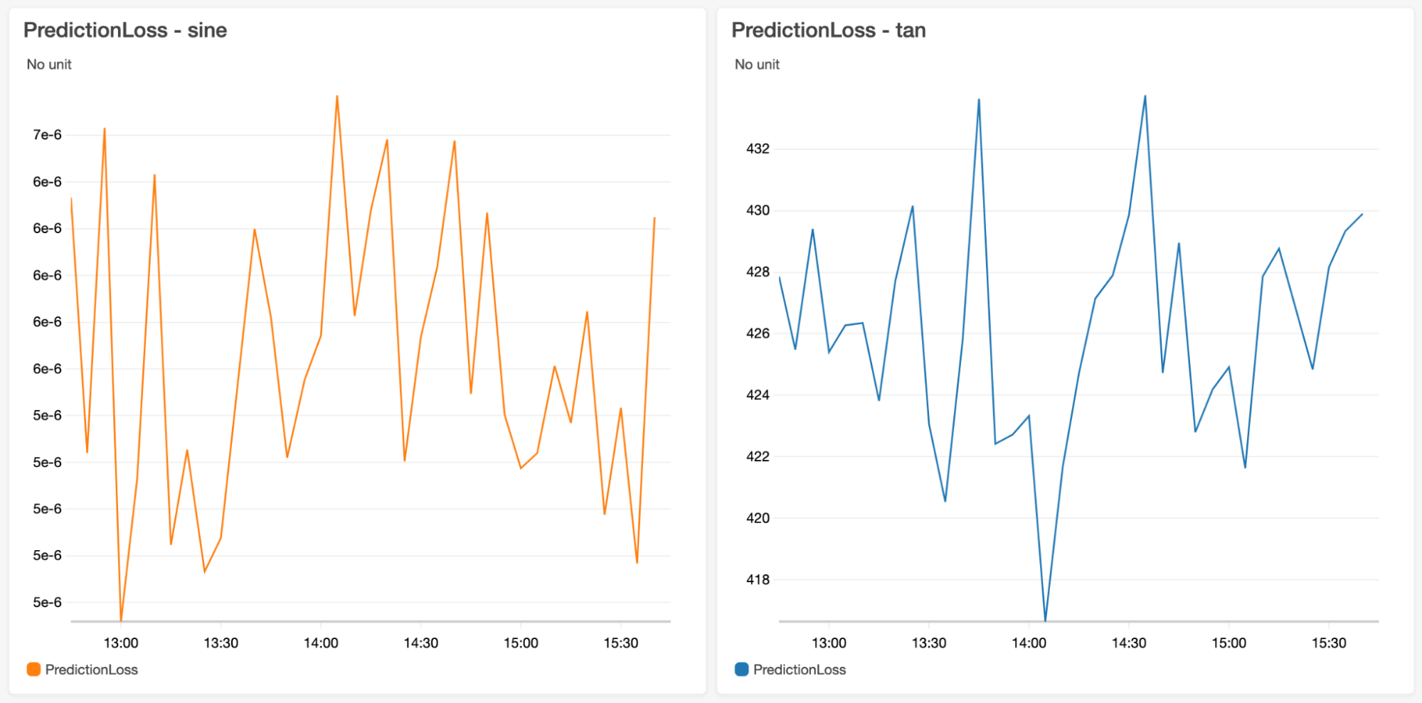
Even though graphs can help a lot with understanding metrics, they aren’t sufficient on their own. You still need experience and statistical knowledge. Consider the two graphs below. The only thing that is obvious from these graphs is that the loss fluctuates a lot. If there’s a distribution shift in any of these two graphs, I can’t tell. It’s easier to plot a graph to draw a wiggling line than to understand what this wiggly line means.

Graphs are useful for making sense of numbers, but they aren’t sufficient.

Excessive metrics and dashboard can also be counterproductive, a phenomenon known as dashboard rot. It’s important to pick the right metrics or abstract out lower-level metrics to compute higher-level signals that make better sense for your specific tasks.

Alerts

When our monitoring system detects something suspicious, it’s necessary to alert the right people about it. An alert consists of the following three components.

1. An alert policy that describes the condition for an alert. You might want to create an alert when a metric breaches a threshold, optionally over a certain duration. For example, you might want to be notified when a model’s accuracy is under 90%, or that the HTTP response latency is higher than a second for at least ten minutes.
2. Notification channels that describe who is to be notified when the condition is met. The alerts will be shown in the monitoring service you employ, such as AWS Cloudwatch or GCP Cloud Monitoring, but you also want to reach responsible people when they’re not on these monitoring services. For example, you might configure your alerts to be sent to an email address such as [email protected], to post to a Slack channel such as #mlops-monitoring or to PagerDuty.

3. A description of the alert to help the alerted person understand what’s going on. The description should be as detailed as possible, such as:

   ## Recommender model accuracy below 90%

   ${timestamp}: This alert originated from the service ${service-name}

   Depending on the audience of the alert, it’s often necessary to make the alert actionable by providing mitigation instructions or a runbook, a compilation of routine procedures and operations that might help with handling the alert.

Alert fatigue is a real phenomenon, as discussed previously in this lecture. Alert fatigue can be demoralizing — nobody likes to be awakened in the middle of the night for something outside of their responsibilities. It’s also dangerous — being exposed to trivial alerts can desensitize people to critical alerts. It’s important to set meaningful conditions so that only critical alerts are sent out.

Observability

Since the mid 2010s, the industry has started embracing the term observability instead of monitoring. Monitoring makes no assumption about the relationship between the internal state of a system and its outputs. You monitor the external outputs of the system to figure out when something goes wrong inside the system — there’s no guarantee that the external outputs will help you figure out what goes wrong.

In the early days of software deployment, software systems were simple enough that monitoring external outputs was sufficient for software maintenance. A system used to consist of only a few components, and a team used to have control over the entire codebase. If something went wrong, it was possible to make changes to the system to test and figure out what went wrong.

However, software systems have grown significantly more complex over the last decade. Today, a software system consists of many components. Many of these components are services run by other companies — cue all cloud native services — which means that a team doesn’t even have control of the inside of all the components of their system. When something goes wrong, a team can no longer just break apart their system to find out. The team has to rely on external outputs of their system to figure out what’s going on internally.

Observability is a term used to address this challenge. It’s a concept drawn from control theory, and refers to bringing “better visibility into understanding the complex behavior of software using [outputs] collected from the system at run time.⁴⁸”

Note: A system’s outputs collected at run time are also called telemetry. Telemetry is another term that has emerged in the software monitoring industry over the last decade. The word “telemetry” comes from the Greek roots “tele” meaning “remote”, and “metron”, meaning “measure”. So telemetry basically means “remote measures”. In the monitoring context, it refers to logs and metrics collected from remote components such as cloud services or applications run on customer devices.

In other words, observability makes an assumption stronger than traditional monitoring: that the internal states of a system can be inferred from knowledge of its external outputs. Internal states can be current states, such as “the GPU utilization right now”, and historical states, such as “the average GPU utilization over the last day.”

When something goes wrong with an observable system, we should be able to figure out what went wrong by looking at the system’s logs and metrics without having to ship new code to the system. Observability is about instrumenting your system in a way to ensure that sufficient information about a system’s run time is collected and analyzed.

Monitoring centers around metrics, and metrics are usually aggregated. Observability allows more fine-grain metrics, so that you can know not only when a model’s performance degrades but also for what types of inputs or what subgroups of users or over what period of time the model degrades. For example, you should be able to query your logs for the answers to the questions like: “show me all the users for which model A returned wrong predictions over the last hour, grouped by their zip codes” or “show me the outliers requests in the last 10 minutes” or “show me all the intermediate outputs of this input through the system”. To achieve this, you need to have logged your system’s outputs using tags and other identifying keywords to allow these outputs to later be sliced and diced along different dimensions of your data.

In ML, observability encompasses interpretability. Interpretability helps us understand how an ML model works, and observability helps us understand how the entire ML system, which includes the ML model, works. For example, when a model’s performance degrades over the last hour, being able to interpret which feature contributes the most to all the wrong predictions made over the last hour will help with figuring out what went wrong with the system and how to fix it.

In this section, we’ve discussed multiple aspects of monitoring, from what data to monitor, what metrics to keep track of, to different tools for monitoring and observability. Even though monitoring is a powerful concept, it’s inherently passive. You wait for a shift to happen to detect it. Monitoring helps unearth the problem without correcting it. In the next section, we’ll introduce continual learning, a paradigm that can actively help you update your models to address shifts.

Acknowledgment

I’d like to thank Han-chung Lee, Thomas Dietterich, Luke Metz, Irené Tematelewo, Zach Nussbaum, Zhenzhong Xu, Shreya Shankar, and Jill Leonard for your amazing feedback!

Notes

If you want to learn any of the above topics, join our Discord chat. We’ll be sharing learning resources and strategies. We might even host learning sessions and discussions if there’s interest. Serious learners only!

1. This is one of the reasons why many companies are hesitant to use products by small startups, and why many companies prefer to use open-source software. When a product you use is no longer maintained by its creators, if that product is open-source, at least you’ll be able to access the codebase and maintain it yourself. ↩

2. Cosmic rays can cause your hardware to break down. ↩

3. A non-ML failure might still be indirectly due to ML. For example, a server can crash for non-ML systems, but because ML systems tend to require more compute power, it might cause this server to crash more often. ↩

4. The peak of my career: Elon Musk agreed with me. ↩

5. Back when in-person academic conferences were still a thing, I often heard researchers arguing about whose models can generalize better. “My model generalizes better than your model” is the ultimate flex. ↩

6. Machine Learning in Non-Stationary Environments: Introduction to Covariate Shift Adaptation (Sugiyama and Kawanabe, The MIT Press 2012) ↩

7. Limits to Growth: Can AI’s Voracious Appetite for Data Be Tamed? (John Mcquaid, Undark 2021) ↩

8. The CTO of a monitoring service company told me that in his estimate, 80% of the drifts captured by his service are caused by human errors. ↩

9. This means the self-driving car is a bit safer than an average human driver. As of 2019, the ratio of traffic-related fatalities per 100,000 licensed drivers was 15.8, or 0.0158%. ↩

10. Edge Cases For Self Driving Cars – Rodney Brooks (2017) ↩

11. Whether Those Endless Edge Or Corner Cases Are The Long-Tail Doom For AI Self-Driving Cars (Forbes, 2021) ↩

12. ​​Self-driving cars will be shaped by simulated, location data (Protocol, 2021) ↩

13. eDiscovery, or electronic discovery, refers to discovery in legal proceedings such as litigation, government investigations, or Freedom of Information Act requests, where the information sought is in electronic format. ↩

14. Degenerate Feedback Loops in Recommender Systems (Jiang et al., 2019) ↩

15. This is related to “survivorship bias”. ↩

16. Beyond NDCG: behavioral testing of recommender systems with RecList (Chia et al., 2021) ↩

17. Why TikTok made its user so obsessive? The AI Algorithm that got you hooked (Catherine Wang, 2020) ↩

18. Improving Aggregate Recommendation Diversity Using Ranking-Based Techniques (Adomavicius et al., 2011) ↩

19. Incremental Learning from Noisy Data (Schlimmer and Granger, 1986) ↩

20. You might wonder what about the case when P(X|Y) changes but P(Y) remains the same, as in the second decomposition. I’ve never encountered any research in this setting. I asked a couple of researchers who specialize in data shifts about it and they also told me that setting would be too difficult to study. ↩

21. An introduction to domain adaptation and transfer learning (Kouw and Loog, 2018) ↩

22. Breast Cancer Risk in American Women (National Cancer Institute) ↩

23. Covariate shift by kernel mean matching (Gretton et al., Journal of Machine Learning Research 2009) ↩

24. Machine Learning in Non-Stationary Environments: Introduction to Covariate Shift Adaptation (Sugiyama and Kawanabe, The MIT Press 2012) ↩

25. Rethinking Importance Weighting for Deep Learning under Distribution Shift (Fang et al., NeurIPS Proceedings 2020) ↩

26. Covariate shift by kernel mean matching (Gretton et al., Journal of Machine Learning Research 2009) ↩

27. You can think of this as the case where both P(X) and P(Y|X) change. ↩

28. If you use a neural network using softmax as your last layer for your classification tax. The dimension of this softmax layer is [number_of_hidden_units x number_of_clases]. When the number of classes changes, the number of parameters in your softmax layer changes. ↩

29. As Han-chung Lee, one early reviewer, pointed out, this is also because smaller companies don’t have enough data on their models. When you don’t have a lot of data, it’s better to have a time-based regimen than to overfit your regime to insufficient data. ↩

30. As a reminder, accuracy-related metrics include accuracy, F1 score, recall, AUC-ROC, etc. ↩

31. You don’t need ground truth labels if you use an unsupervised learning method, but the vast majority of applications today are supervised. ↩

32. Hamel Husain gave a great lecture on why TensorFlow Extended’s skew detection is so bad for CS 329S: Machine Learning Systems Design (Stanford, 2022). You can find the video here. ↩

33. Handbook of Methods of Applied Statistics, Volume 1 (Chakravart, Laha, and Roy, 1967). ↩

34. Beware the Kolmogorov-Smirnov test! (Feigelson and Babu, Center for Astrostatistics, Penn State University) ↩

35. Data validation for machine learning (Breck et al., Proceedings of SysML 2019) ↩

36. A pdf-Free Change Detection Test Based on Density Difference Estimation (Bu et al., 2016). The authors claim that the method works on multidimensional inputs. ↩

37. Failing Loudly: An Empirical Study of Methods for Detecting Dataset Shift (Rabanser et al., 2018) ↩

38. Early Drift Detection Method (Baena-Garcia et al., 2006) ↩

39. Real-time Drift Detection on Time-series Data (Ramanan et al., 2021) ↩

40. I’m working on a solution that can handle the minute granularity level. ↩

41. Thanks Goku Mohandas for sharing this tip on the MLOps Discord server. ↩

42. Detecting and Correcting for Label Shift with Black Box Predictors (Lipton et al., 2018) ↩

43. Some monitoring vendors claim that their solutions are able to detect not only when your model should be retrained, but also what data to retrain on. I haven’t been able to verify the validity of these claims. ↩

44. Failing Loudly: An Empirical Study of Methods for Detecting Dataset Shift (Rabanser et al., 2018) ↩

45. Observability — A 3-Year Retrospective (Charity Majors, The New Stack 2019) ↩

46. Log Management Market Size, Share and Global Market Forecast to 2026 (MarketsandMarkets, 2021) ↩

47. For readers unfamiliar with stream processing, please refer to the Batch Processing vs. Stream Processing section in lecture 8. ↩

48. Towards Observability Data Management at Scale (Karumuri et al., ACM SIGMOD Record, Volume 49, Issue 4, 2020) ↩